Singing the Bayesian Beginner Blues
By Julia Silge
September 28, 2016
Earlier this week, I published a post about song lyrics and how different U.S. states are mentioned at different rates, and at different rates relative to their populations. That was a very fun post to work on, but you can tell from that paragraph near the end that I am a little bothered by the uncertainty involved in calculating the rates by just dividing two numbers. David Robinson suggested on Twitter that I might try using empirical Bayes methods to estimate the rates. I am a newcomer to Bayesian methods but this idea makes a lot of sense in this context, so let’s see what we can do!
Getting Started
The analysis here borrows very heavily from two of Dave’s posts from last year. To start out, what are the values that we are dealing with? (I have hidden the code that downloads/calculates these values, but you can see the entire R Markdown file here.)
state_counts %>%
    arrange(desc(rate)) %>%
    top_n(10)
## # A tibble: 10 × 4
##      state_name  pop2014     n         rate
##          <fctr>    <dbl> <dbl>        <dbl>
## 1        Hawaii  1392704     6 4.308166e-06
## 2   Mississippi  2984345    10 3.350819e-06
## 3      New York 19594330    64 3.266251e-06
## 4       Alabama  4817678    12 2.490826e-06
## 5       Georgia  9907756    22 2.220483e-06
## 6     Tennessee  6451365    14 2.170083e-06
## 7       Montana  1006370     2 1.987341e-06
## 8      Nebraska  1855617     3 1.616713e-06
## 9      Kentucky  4383272     7 1.596981e-06
## 10 North Dakota   704925     1 1.418591e-06
We have, for each state here, the population in the state, the number of times it was mentioned in a song, and the rate of mentions per population (just the previous two numbers divided by each other). The reason I was uncomfortable here is that some states were mentioned so few times (like Hawaii and Montana!) and it is surely true that the rates calculated here have very different uncertainty intervals from state to state.
Bayesian Who?!
This is where Bayesian methods come in. We can use Bayesian methods to a) estimate the rate itself and b) estimate credible intervals. For a really wonderful explanation of how Bayesian models work, I will point you to Rasmus Bååth’s post about whether his wife is pregnant or not. He posted that last year not too long after Dave posted some of his baseball/Bayes posts, at which time I started to think, “Maybe this Bayes stuff does actually make sense.” To use a Bayesian method, we need to choose a prior probability distribution for what we want to estimate; this is what we believe about the quantity before evidence is taken into account. What makes empirical Bayes “empirical” is that the prior probability distribution is taken from the data itself; we will plot the actual distribution of rates (mentions per population) and use that distribution as our prior.
ggplot(state_counts, aes(rate)) +
    geom_histogram(binwidth = 2e-7, alpha = 0.8, fill = "midnightblue") +
    labs(x = "rate of mentions per population") +
    theme_minimal(base_family = "RobotoCondensed-Regular")
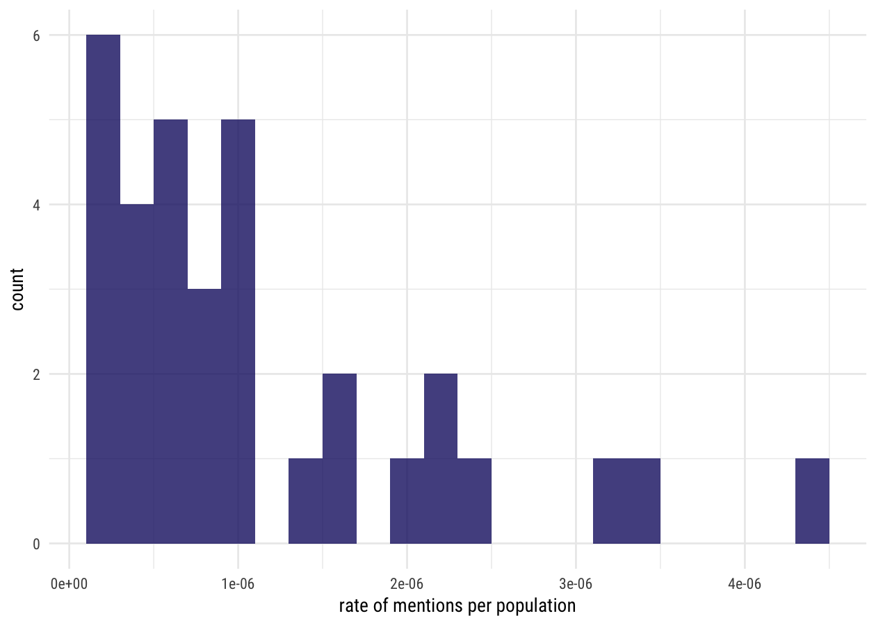
Hmmmmm, that’s not so great, is it? There are only 50 states and not all of them were mentioned in this lyrics data set at all. But we will merrily push forward and calculate a prior probability distribution from this. Let’s fit a beta distribution to this to use as our prior. I’m going to use the method of moments to fit a beta distribution.
x <- state_counts$n / state_counts$pop2014
mu <- mean(x)
sigma2 <- var(x)
alpha0 <- ((1 - mu) / sigma2 - 1 / mu) * mu^2
beta0 <- alpha0 * (1 / mu - 1)
Now let’s plot this.
ggplot(state_counts) +
    geom_histogram(aes(rate, y = ..density..), binwidth = 2e-7, alpha = 0.8, fill = "midnightblue") +
    stat_function(fun = function(x) dbeta(x, alpha0, beta0),
                  color = "red", size = 1) +
    labs(x = "rate of mentions per population") +
    theme_minimal(base_family = "RobotoCondensed-Regular")
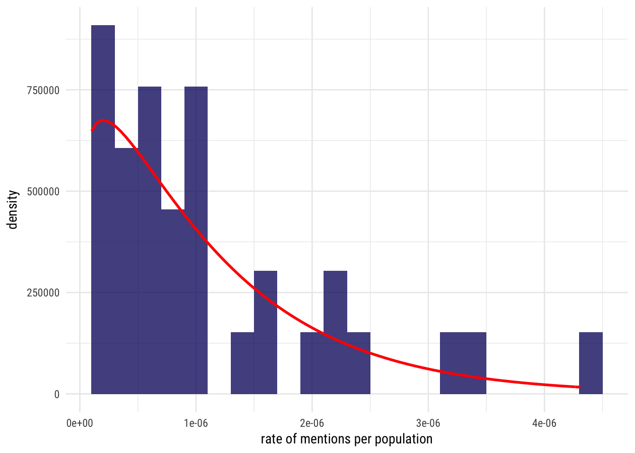
That’s not… too awful, I hope. Remember, what this is supposed to be is our belief about the distribution of rates before evidence from individual states is taken into account. I would buy this in a general sense; there a few states that are mentioned many times and many states that are mentioned a few times.
And that’s it! We have a prior.
Calculating the Empirical Bayes Estimate
Now that we have a prior probability distribution, we use Bayes' theorem to calculate a posterior estimate for each state’s rate. It’s not very difficult math.
state_counts <- state_counts %>%
    mutate(rate_estimate = 1e6*(n + alpha0) / (pop2014 + alpha0 + beta0),
           rate = 1e6*rate)

state_counts
## # A tibble: 33 × 5
##    state_name  pop2014     n      rate rate_estimate
##        <fctr>    <dbl> <dbl>     <dbl>         <dbl>
## 1     Alabama  4817678    12 2.4908265     2.2473115
## 2     Arizona  6561516     4 0.6096152     0.6838013
## 3    Arkansas  2947036     1 0.3393240     0.5519852
## 4  California 38066920    34 0.8931639     0.8999236
## 5    Colorado  5197580     3 0.5771917     0.6730431
## 6     Florida 19361792     4 0.2065924     0.2552334
## 7     Georgia  9907756    22 2.2204826     2.1161297
## 8      Hawaii  1392704     6 4.3081660     2.9387203
## 9       Idaho  1599464     1 0.6252094     0.8315038
## 10   Illinois 12868747     6 0.4662459     0.5177696
## # ... with 23 more rows
How do the two values compare?
library(ggrepel)
ggplot(state_counts, aes(rate, rate_estimate, color = n)) +
    geom_abline(intercept = 0, slope = 1, color = "gray70", linetype = 2) +
    geom_text_repel(aes(label = state_name), color = "black",
                    box.padding = unit(0.5, 'lines'),
                    family = "RobotoCondensed-Regular") +
    geom_point(size = 4) +
    scale_color_gradient(low = "midnightblue", high = "pink",
                         name="Number\nof songs") +
    labs(title = "States in Song Lyrics with Empirical Bayes",
         subtitle = "States like Montana and Hawaii (high rates, few mentions) are shifted the most",
         x = "Measured rate of mentions per million population",
         y = "Empirical Bayes estimate of rate per million population") +
    theme_minimal(base_family = "RobotoCondensed-Regular") +
    theme(plot.title=element_text(family="Roboto-Bold"))
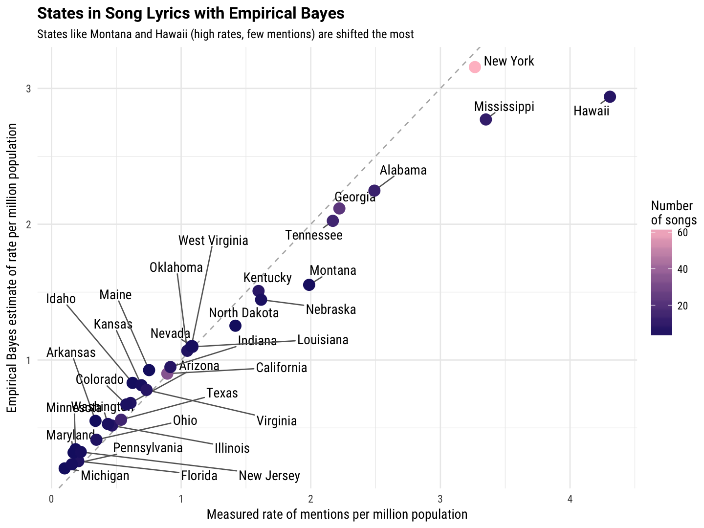
Notice that the states that were mentioned the highest number of times are closest to the line, i.e., the empirical Bayes method here did not change the value that much. It is only for states that were mentioned in a few songs that the two values are quite different. Notice that the high rates were shifted to lower values and the low rates were shifted to (slightly) higher values.
What Is the Posterior Distribution for Each State?
We calculated an empirical Bayes estimate for each rate above, but we can actually calculate the full posterior probability distribution for each state. What are $\alpha$ and $\beta$ for each state?
state_counts <- state_counts %>%
    mutate(alpha1 = n + alpha0,
           beta1 = pop2014 - n + beta0)

state_counts
## # A tibble: 33 × 7
##    state_name  pop2014     n      rate rate_estimate    alpha1    beta1
##        <fctr>    <dbl> <dbl>     <dbl>         <dbl>     <dbl>    <dbl>
## 1     Alabama  4817678    12 2.4908265     2.2473115 13.212753  5879346
## 2     Arizona  6561516     4 0.6096152     0.6838013  5.212753  7623192
## 3    Arkansas  2947036     1 0.3393240     0.5519852  2.212753  4008715
## 4  California 38066920    34 0.8931639     0.8999236 35.212753 39128566
## 5    Colorado  5197580     3 0.5771917     0.6730431  4.212753  6259257
## 6     Florida 19361792     4 0.2065924     0.2552334  5.212753 20423468
## 7     Georgia  9907756    22 2.2204826     2.1161297 23.212753 10969414
## 8      Hawaii  1392704     6 4.3081660     2.9387203  7.212753  2454378
## 9       Idaho  1599464     1 0.6252094     0.8315038  2.212753  2661143
## 10   Illinois 12868747     6 0.4662459     0.5177696  7.212753 13930421
## # ... with 23 more rows
Let’s plot a few of these to see what they look like.
library(broom)
counts_beta <- state_counts %>%
    arrange(desc(rate_estimate)) %>%
    top_n(5, rate_estimate) %>%
    inflate(x = seq(1e-7, 5e-6, 2e-8)) %>%
    ungroup() %>%
    mutate(density = dbeta(x, alpha1, beta1))

ggplot(counts_beta, aes(x, density, color = state_name)) +
    geom_line(size = 1.2, alpha = 0.8) +
    stat_function(fun = function(x) dbeta(x, alpha0, beta0),
                  lty = 2, color = "black") +
    labs(x = "Rate of mentions per population",
         y = "Density",
         title = "Prior and Posterior Distributions",
         subtitle = "The posterior distribution for a few example states are shown\nThe prior distribution is shown as a dashed line") +
    theme_minimal(base_family = "RobotoCondensed-Regular") +
    theme(plot.title=element_text(family="Roboto-Bold")) +
    theme(legend.title=element_blank())
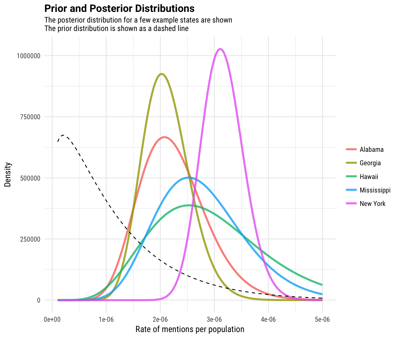
Notice that New York, which was mentioned in many songs, has a narrow posterior probability distribution; we have more precise knowledge about the rate for New York. Hawaii, by contrast, has a broad probability distribution; we have less precise knowledge about the rate for Hawaii, because Hawaii was only mentioned in a few songs!
We can use these posterior probability distributions to calculate credible intervals, an estimate of how uncertain each of these measurements is, analogous to a confidence interval. (BUT SO DIFFERENT, everyone tells me. ON A PHILOSOPHICAL LEVEL.)
state_counts <- state_counts %>%
    mutate(low  = 1e6*qbeta(.025, alpha1, beta1),
           high = 1e6*qbeta(.975, alpha1, beta1))
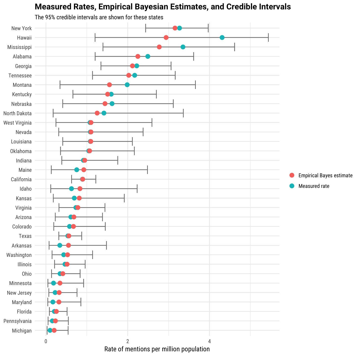
These are 95% credible intervals. Let’s check them out!
library(tidyr)
state_counts %>%
    arrange(desc(rate_estimate)) %>%
    mutate(state_name = factor(state_name, levels = rev(unique(state_name)))) %>%
    select(state_name, 'Measured rate' = rate, 'Empirical Bayes estimate' = rate_estimate, low, high) %>%
    gather(type, rate, `Measured rate`, `Empirical Bayes estimate`) %>%
    ggplot(aes(rate, state_name, color = type)) +
    geom_errorbarh(aes(xmin = low, xmax = high), color = "gray50") +
    geom_point(size = 3) +
    xlim(0, NA) +
    labs(x = "Rate of mentions per million population",
         y = NULL, title = "Measured Rates, Empirical Bayesian Estimates, and Credible Intervals",
         subtitle = "The 95% credible intervals are shown for these states") +
    theme_minimal(base_family = "RobotoCondensed-Regular") +
    theme(plot.title=element_text(family="Roboto-Bold")) +
    theme(legend.title=element_blank())
The End
The part of this that was the most satisfying was the credible intervals, how big/small they are, and how the plain vanilla rates and empirical Bayes rate estimates are distributed in the credible intervals. It definitely gave me the data intuition warm fuzzies and made a lot of sense. This method is not that hard to implement or understand and was a gratifyingly productive first foray into Bayesian methods. The R Markdown file used to make this blog post is available here. I am very happy to hear feedback or questions!