Reddit Responds to the Election
By Julia Silge
December 6, 2016
It’s been about a month since the U.S. presidential election, with Donald Trump’s victory over Hillary Clinton coming as a surprise to most. Reddit user Jason Baumgartner collected and published every submission and comment posted to Reddit on the day of (and a bit surrounding) the U.S. election; let’s explore this data set and see what kinds of things we can learn.
Data wrangling
This first bit was the hardest part of this analysis for me, probably because I am not the most experienced JSON person out there. At first, I took an approach of reading in the lines of each text file and parsing each JSON object separately. I
complained about this on Twitter and got several excellent recommendations of much better approaches, including using stream_in from the
jsonlite package. This works way better and faster than what I was doing before, and now it is easy!
library(jsonlite)
library(dplyr)

nov8_posts <- stream_in(file("RS_2016-11-08"),
                        verbose = FALSE) %>%
    select(-preview, -secure_media_embed,
           -media, -secure_media, -media_embed)

nov9_posts <- stream_in(file("RS_2016-11-09"),
                        verbose = FALSE) %>%
    select(-preview, -secure_media_embed,
           -media, -secure_media, -media_embed)

posts <- bind_rows(nov8_posts, nov9_posts) %>%
    mutate(created_utc = as.POSIXct(created_utc,
                                    origin = "1970-01-01",
                                    tz = "UTC")) %>%
    filter(created_utc > as.POSIXct("2016-11-08 18:00:00", tz = "UTC"))
Notice here that I am using files from November 8 and 9 in UTC time and I’m filtering out some of the earlier posts. This will end up leaving me with 30 hours of Reddit posts starting at noon on Election Day in the Central Time Zone. Also notice that I am not using the files that include Reddit comments, only the parent submissions. I tried most of the following analysis with both submissions and comments, but the comments dominated the results and included lots of repeated words/phrases that obscured what we would like to see. For the approach I am taking here, it worked better to just use submissions.
Finding the words
The submissions include a title and sometimes also some text; sometimes Reddit posts are just the title. Let’s use unnest_tokens from the
tidytext package to identify all the words in the title and text fields of the submissions and organize them into a tidy data structure.
library(tidytext)

posts <- bind_rows(
    posts %>%
        unnest_tokens(word, title),
    posts %>%
        unnest_tokens(word, selftext)) %>%
    select(created_utc, subreddit, url, word)

head(posts)
##           created_utc  subreddit
## 1 2016-11-08 18:00:01 Ebay_deals
## 2 2016-11-08 18:00:01 Ebay_deals
## 3 2016-11-08 18:00:01 Ebay_deals
## 4 2016-11-08 18:00:01 Ebay_deals
## 5 2016-11-08 18:00:01 Ebay_deals
## 6 2016-11-08 18:00:01 Ebay_deals
##                                                 url   word
## 1 https://www.pinterest.com/pin/724587027517110980/ marble
## 2 https://www.pinterest.com/pin/724587027517110980/   grey
## 3 https://www.pinterest.com/pin/724587027517110980/ single
## 4 https://www.pinterest.com/pin/724587027517110980/ double
## 5 https://www.pinterest.com/pin/724587027517110980/  queen
## 6 https://www.pinterest.com/pin/724587027517110980/   king
dim(posts)
## [1] 17652591 4
That’s… almost 18 million rows. People on Reddit are busy.
Which words changed in frequency the fastest?
Right now we have a data frame that has each word on its own row, with an id (url), the time when it was posted, and the subreddit it came from. Let’s use dplyr operations to calculate how many times each word was mentioned in a particular unit of time, so we can model the change with time. We will calculate minute_total, the total words posted in that time unit so we can compare across times of day when people post different amounts, and word_total, the number of times that word was posted so we can filter out words that are not used much.
library(lubridate)
library(stringr)

words_by_minute <- posts %>%
    filter(str_detect(word, "[a-z]")) %>%
    anti_join(data_frame(word = c("ref"))) %>%
    mutate(created = floor_date(created_utc, unit = "30 minutes")) %>%
    distinct(url, word, .keep_all = TRUE) %>%
    count(created, word) %>%
    ungroup() %>%
    group_by(created) %>%
    mutate(minute_total = sum(n)) %>%
    group_by(word) %>%
    mutate(word_total = sum(n)) %>%
    ungroup() %>%
    rename(count = n) %>%
    filter(word_total > 500)

head(words_by_minute)
## # A tibble: 6 × 5
##               created  word count minute_total word_total
##                <dttm> <chr> <int>        <int>      <int>
## 1 2016-11-08 18:00:00 1080p    20       231072        652
## 2 2016-11-08 18:00:00  16gb    11       231072        559
## 3 2016-11-08 18:00:00   1st    20       231072        758
## 4 2016-11-08 18:00:00   2nd    21       231072        893
## 5 2016-11-08 18:00:00    2x    14       231072        722
## 6 2016-11-08 18:00:00    3d    12       231072        546
This is the data frame we can use for modeling. We can use nest from tidyr to make a data frame with a list column that contains the little miniature data frames for each word and then map from purrr to apply our modeling procedure to each of those little data frames inside our big data frame. Jenny Bryan has put together
some resources on using purrr with list columns this way. This is count data (how many words were posted?) so let’s use glm for modeling.
library(tidyr)
library(purrr)

nested_models <- words_by_minute %>%
    nest(-word) %>%
    mutate(models = map(data, ~ glm(cbind(count, minute_total) ~ created, .,
                                    family = "binomial")))
Now we can use tidy from broom to pull out the slopes for each of these models and find the important ones.
library(broom)

slopes <- nested_models %>%
  unnest(map(models, tidy)) %>%
  filter(term == "created")
Which words decreased in frequency of use the fastest during Election Day? Which words increased in use the fastest?
slopes %>%
    arrange(estimate)
## # A tibble: 891 × 6
##        word    term      estimate    std.error statistic       p.value
##       <chr>   <chr>         <dbl>        <dbl>     <dbl>         <dbl>
## 1   polling created -2.195136e-05 1.059199e-06 -20.72449  2.083382e-95
## 2     fraud created -2.022229e-05 1.335022e-06 -15.14753  7.866753e-52
## 3    voting created -1.788212e-05 5.644046e-07 -31.68316 2.651017e-220
## 4    ballot created -1.745250e-05 1.114699e-06 -15.65670  2.990299e-55
## 5        fl created -1.743009e-05 1.211878e-06 -14.38271  6.644389e-47
## 6   florida created -1.712721e-05 6.055286e-07 -28.28472 5.327752e-176
## 7      poll created -1.688132e-05 1.039083e-06 -16.24637  2.369894e-59
## 8     voter created -1.675932e-05 9.359359e-07 -17.90649  1.049562e-71
## 9     polls created -1.615500e-05 7.058145e-07 -22.88845 6.054992e-116
## 10 virginia created -1.493344e-05 1.435504e-06 -10.40293  2.404218e-25
## # ... with 881 more rows
slopes %>%
    arrange(desc(estimate))
## # A tibble: 891 × 6
##        word    term     estimate    std.error statistic       p.value
##       <chr>   <chr>        <dbl>        <dbl>     <dbl>         <dbl>
## 1   trump’s created 1.758326e-05 1.430901e-06 12.288244  1.047563e-34
## 2      flex created 1.416875e-05 1.290926e-06 10.975647  5.004609e-28
## 3     elect created 1.390813e-05 8.378822e-07 16.599146  7.068929e-62
## 4        da created 1.281702e-05 1.037396e-06 12.354986  4.578350e-35
## 5  congress created 1.225188e-05 1.280413e-06  9.568696  1.082627e-21
## 6   trump's created 1.200055e-05 5.499216e-07 21.822297 1.425196e-105
## 7  policies created 1.156944e-05 1.276465e-06  9.063655  1.261512e-19
## 8  liberals created 1.151984e-05 1.151751e-06 10.002020  1.493199e-23
## 9   climate created 1.092999e-05 1.269681e-06  8.608452  7.405384e-18
## 10   policy created 9.879997e-06 1.038524e-06  9.513494  1.843631e-21
## # ... with 881 more rows
Let’s plot these words.
top_slopes <- slopes %>%
    top_n(10, estimate)

words_by_minute %>%
    inner_join(top_slopes, by = "word") %>%
    mutate(created = with_tz(created, tz = "America/Chicago")) %>%
    ggplot(aes(created, count/minute_total, color = word)) +
    geom_line(alpha = 0.8, size = 1.3) +
    labs(x = "Time (Central Time Zone)", y = "Word frequency",
         subtitle = "Words associated with Trump and policies increased in frequency",
         title = "Trending words on Reddit on Election Day")
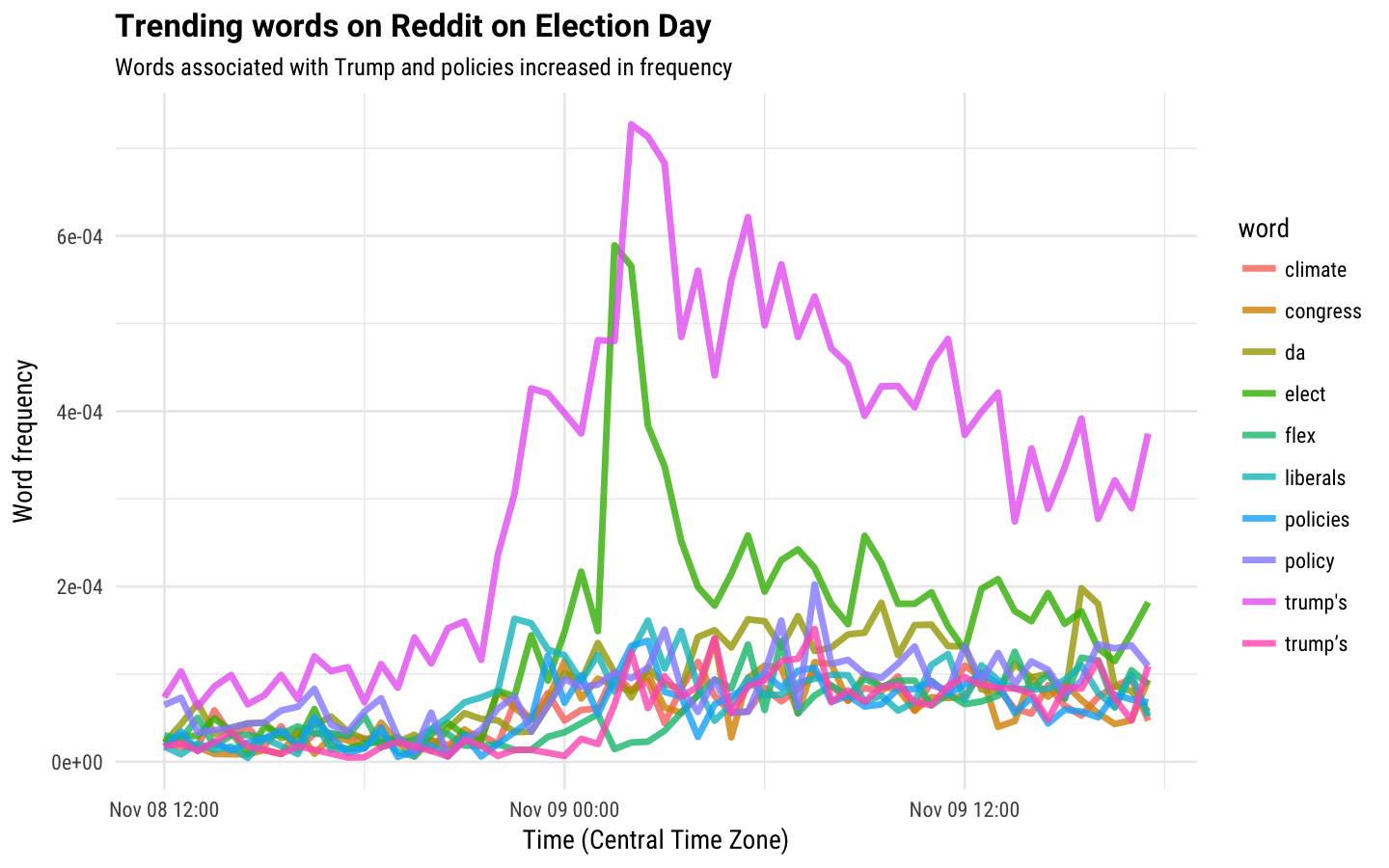
There are lots of election-related words here, like “elect”, “liberals”, and “policies”. In fact, I think all of these words are conceivably related to the election with the exception of “flex”. I looked at some of the posts with “flex” in them and they were in fact not election-related. I had a hard time deciphering what they were about, but my best guess is either a) fantasy football or b) some kind of gaming. Why do we see “Trump’s” on this plot twice? It is because there is more than one way of encoding an apostrophe. You can see it on the legend if you look closely.
We don’t see Trump’s name by itself on this plot. How far off from being a top word, by my definition here, was it?
slopes %>%
    filter(word == "trump")
## # A tibble: 1 × 6
##    word    term     estimate    std.error statistic      p.value
##   <chr>   <chr>        <dbl>        <dbl>     <dbl>        <dbl>
## 1 trump created 2.328675e-06 1.512196e-07   15.3993 1.654546e-53
Trump must have been being discussed at a high level already, so the change was not as big as for the word “Trump’s”.
What about the words that dropped in use the most during this day?
low_slopes <- slopes %>%
    top_n(-10, estimate)

words_by_minute %>%
    inner_join(low_slopes, by = "word") %>%
    mutate(created = with_tz(created, tz = "America/Chicago")) %>%
    ggplot(aes(created, count/minute_total, color = word)) +
    geom_line(alpha = 0.8, size = 1.3) +
    labs(x = "Time (Central Time Zone)", y = "Word frequency",
         subtitle = "Word associated with voting and polls decreased in frequency",
         title = "Trending words on Reddit on Election Day")
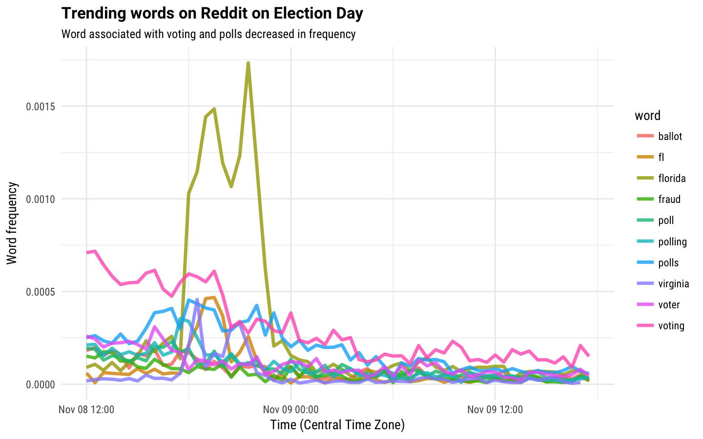
These are maybe even more interesting to me. Look at that spike for Florida the night of November 8 when it seemed like there might be flashbacks to 2000 or something. And people’s interest in discussing voters/voting, polls/polling, and fraud dropped off precipitously as Trump’s victory became obvious.
Which subreddits demonstrated the most change in sentiment?
We have looked at which words changed most quickly in use on Election Day; now let’s take a look at changes in sentiment. Are there subreddits that exhibited changes in sentiment over the course of this time period? To look at this, we’ll take a bigger time period (2 hours instead of 30 minutes) since the words with measured sentiment are only a subset of all words. Much of the rest of these dplyr operations are similar. We can use inner_join to do the sentiment analysis, and then calculate the sentiment content of each board in each time period.
sentiment_by_minute <- posts %>%
    mutate(created = floor_date(created_utc, unit = "2 hours")) %>%
    distinct(url, word, .keep_all = TRUE) %>%
    ungroup() %>%
    count(subreddit, created, word) %>%
    group_by(created, subreddit) %>%
    mutate(minute_total = sum(n)) %>%
    group_by(subreddit) %>%
    mutate(subreddit_total = sum(n)) %>%
    ungroup() %>%
    filter(subreddit_total > 1000) %>%
    inner_join(get_sentiments("afinn")) %>%
    group_by(subreddit, created, minute_total) %>%
    summarize(score = sum(n * score)) %>%
    ungroup()

head(sentiment_by_minute)
## # A tibble: 6 × 4
##   subreddit             created minute_total score
##       <chr>              <dttm>        <int> <int>
## 1     1liga 2016-11-08 20:00:00           20     2
## 2     1liga 2016-11-09 02:00:00          135    -7
## 3     1liga 2016-11-09 06:00:00          187    -9
## 4     1liga 2016-11-09 08:00:00          233    -8
## 5     1liga 2016-11-09 10:00:00          155    -2
## 6     1liga 2016-11-09 12:00:00          110    -6
Let’s again use nest, but this time we’ll nest by subreddit instead of word. This sentiment score is not really count data (since it can be negative) so we’ll use regular old lm here.
nested_models <- sentiment_by_minute %>%
    nest(-subreddit) %>%
    mutate(models = map(data, ~ lm(score/minute_total ~ created, .)))
Let’s again use unnest, map, and tidy to extract out the slopes from the linear models.
slopes <- nested_models %>%
  unnest(map(models, tidy)) %>%
  filter(term == "created")
Which subreddits exhibited the biggest changes in sentiment, in either direction?
slopes %>%
    arrange(estimate)
## # A tibble: 64 × 6
##            subreddit    term      estimate    std.error statistic     p.value
##                <chr>   <chr>         <dbl>        <dbl>     <dbl>       <dbl>
## 1        aznidentity created -2.941746e-06 1.129234e-06 -2.605081 0.040386018
## 2             ainbow created -2.576480e-06 8.841939e-07 -2.913932 0.017200835
## 3        TheBluePill created -2.233135e-06 6.868578e-07 -3.251233 0.009977663
## 4    muacjdiscussion created -2.165141e-06 4.838494e-07 -4.474823 0.020801581
## 5            parrots created -2.105393e-06 7.592753e-07 -2.772898 0.024188248
## 6         needadvice created -1.610350e-06 5.277117e-07 -3.051572 0.018542125
## 7        sweepstakes created -1.458346e-06 5.576759e-07 -2.615042 0.022590562
## 8  RandomActsofCards created -1.421334e-06 5.556567e-07 -2.557935 0.026616327
## 9       csgogambling created -1.397576e-06 5.619925e-07 -2.486823 0.027257440
## 10             1liga created -1.305359e-06 4.842398e-07 -2.695688 0.027255456
## # ... with 54 more rows
slopes %>%
    arrange(desc(estimate))
## # A tibble: 64 × 6
##            subreddit    term     estimate    std.error statistic     p.value
##                <chr>   <chr>        <dbl>        <dbl>     <dbl>       <dbl>
## 1  shoudvebeenbernie created 2.792205e-06 7.339321e-07  3.804446 0.008921294
## 2        TheDickShow created 2.189643e-06 7.900087e-07  2.771670 0.019730686
## 3            orlando created 1.860757e-06 7.313366e-07  2.544324 0.034477936
## 4    DoesAnybodyElse created 1.846480e-06 5.773406e-07  3.198251 0.007657351
## 5    playrustservers created 1.553049e-06 5.623340e-07  2.761791 0.032776294
## 6    GoogleCardboard created 1.449634e-06 5.215326e-07  2.779565 0.032015397
## 7    morbidquestions created 1.423202e-06 4.865300e-07  2.925208 0.019138028
## 8          TrueDoTA2 created 1.388537e-06 3.592288e-07  3.865329 0.011816017
## 9        JapanTravel created 1.365982e-06 3.702370e-07  3.689479 0.005001422
## 10           editors created 1.253335e-06 4.080638e-07  3.071420 0.011812188
## # ... with 54 more rows
Let’s plot these!
top_slopes <- slopes %>%
    top_n(10, estimate)

sentiment_by_minute %>%
    inner_join(top_slopes, by = "subreddit") %>%
    mutate(created = with_tz(created, tz = "America/Chicago")) %>%
    ggplot(aes(created, score/minute_total, color = subreddit)) +
    geom_line(alpha = 0.8, size = 1.3) +
    labs(x = "Time (Central Time Zone)", y = "Sentiment score",
         subtitle = "These subreddits increased in sentiment the most",
         title = "Sentiment on Subreddits on Election Day")
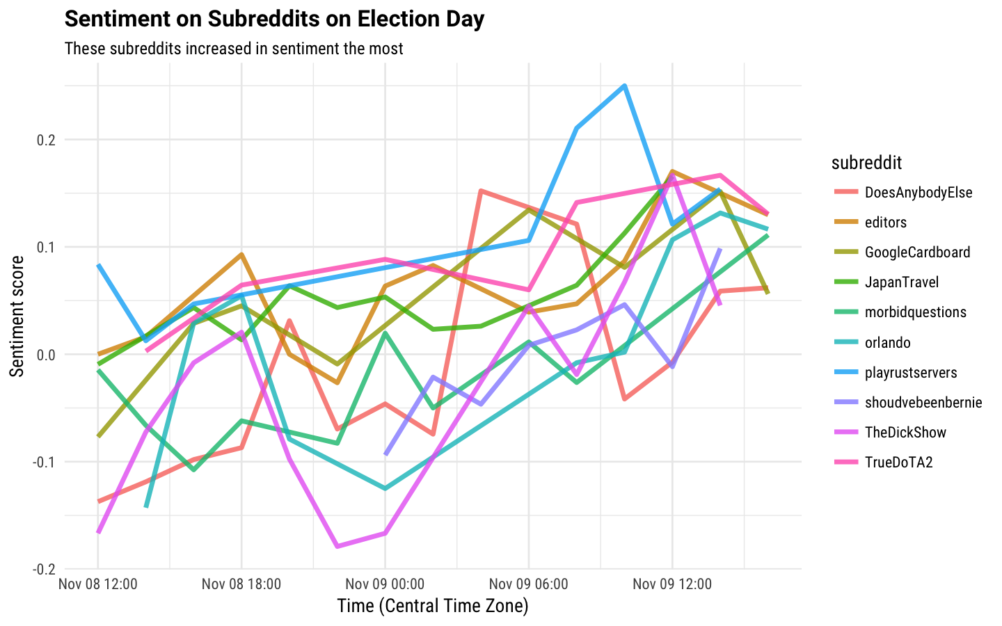
These relationships are much noisier than the relationships with words were, and you might notice that some p-values are getting kind of high (no adjustment for multiple comparisons has been performed). Also, these subreddits are less related to the election than the quickly changing words were. Really only the shouldvebeenbernie subreddit is that political here.
low_slopes <- slopes %>%
    top_n(-10, estimate)

sentiment_by_minute %>%
    inner_join(low_slopes, by = "subreddit") %>%
    mutate(created = with_tz(created, tz = "America/Chicago")) %>%
    ggplot(aes(created, score/minute_total, color = subreddit)) +
    geom_line(alpha = 0.8, size = 1.3) +
    labs(x = "Time (Central Time Zone)", y = "Sentiment score",
         subtitle = "These subreddits decreased in sentiment the most",
         title = "Sentiment on Subreddits on Election Day")
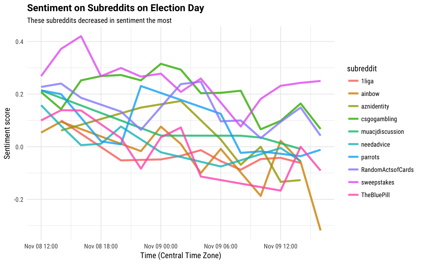
Again, we see that not really any of these are specifically political, although I coudld image that the aznidentity subreddit (Asian identity board) and the ainbow subreddit (LGBT board) could have been feeling down after Trump’s election. The 1liga board is a German language board and ended up here because it used the word “die” a lot. In case you are wondering, the parrots subreddit is, in fact, about parrots; hopefully nothing too terrible was happening to the parrots on Election Day.
Which subreddits have the most dramatic word use?
Those last plots demonstrated with subreddits were changing in sentiment the fastest around the time of the election, but perhaps we would like to know which subreddits used the largest proportion of high or low sentiment words overall during this time period. To do that, we don’t need to keep track of the timestamp of the posts. Instead, we just need to count by subreddit and word, then use inner_join to find a sentiment score.
sentiment_by_subreddit <- posts %>%
    distinct(url, word, .keep_all = TRUE) %>%
    count(subreddit, word) %>%
    ungroup() %>%
    inner_join(get_sentiments("afinn")) %>%
    group_by(subreddit) %>%
    summarize(score = sum(score * n) / sum(n))
I would print some out for you, or plot them or something, but they are almost all extremely NSFW, both the positive and negative sentiment subreddits. I’m sure you can use your imagination.
The End
This is just one approach to take with this extremely extensive data set. There is still lots and lots more that could be done with it. I first saw this data set via Jeremy Singer-Vine’s Data Is Plural newsletter; this newsletter is an excellent resource and I highly recommend it. The R Markdown file used to make this blog post is available here. I am very happy to hear feedback or questions!