If I Loved Natural Language Processing Less, I Might Be Able to Talk About It More
By Julia Silge
March 18, 2016
In my last post, I did some natural language processing and sentiment analysis for Jane Austen’s most well-known novel, Pride and Prejudice. It was just so much fun that I wanted to extend some of that work and compare across her body of writing.
I decided to make an R package for her texts, for easy access for myself and anybody else who would like to do some text analysis on a nice sample of prose. The package is
available on Github and can be installed via devtools.
library(devtools)
install_github("juliasilge/janeaustenr")
library(janeaustenr)
You can read more details in the documentation and README, but the package contains the full text of the 6 completed, published novels of Jane Austen. The UTF-8 plain text for each novel was sourced from
Project Gutenberg and then I processed them a bit to remove the Project Gutenberg headers and footers as well as blank lines and NA lines, etc. Now they are all ready for text analysis. Each text is in a character vector with elements of about 70 characters. Let’s load them, along with the libraries we’ll need for this analysis.
library(dplyr)
library(stringr)
library(syuzhet)
library(ggplot2)
library(viridis)
data(sensesensibility)
data(prideprejudice)
data(mansfieldpark)
data(emma)
data(northangerabbey)
data(persuasion)
As I was working on this package, I discovered that three of the novels are already available within the
stylo package; this package was built for stylometric analysis of text (that sounds SO FUN…) and the texts for three of Jane Austen’s books are in the novels data set in that package, along with 6 novels by the Brontë sisters. Undeterred, I decided to put together this package anyway with all of Jane Austen’s completed published works. The data objects appear to be quite similar, however, as we both used the Project Gutenberg UTF-8 plain text files and performed similar processing.
I have been pondering doing something more ambitious along these lines. Wouldn’t it be great to have a really big sample of books easily accessible in R? I am still considering how to implement such a thing, though. Some of the processing to get these texts into an R package is easy to automate, but some of it isn’t; the Project Gutenberg headers and footers seem to not be standard in length, etc. Matthew Jockers talks about using a corpus of tens of thousands of novels, but doesn’t give information on how to access a publicly available version of this corpus. We’ll see!
Options for Sentiment Analysis
Now that we have the texts for Jane Austen’s novels, let’s concatenate the ~70-character lines into larger chunks. I got a couple of suggestions to avoid my use of a for loop for chunking the text in my last post. My favorite is probably the dplyr one shared by the
knowledgeable/generous David Robinson. Much nicer! Then let’s calculate the sentiment for each chunk of text. This is in a function because we are going to use this a bunch of times.
process_sentiment <- function (rawtext, mymethod) {
        chunkedtext <- data_frame(x = rawtext) %>%
                group_by(linenumber = ceiling(row_number() / 10)) %>%
                summarize(text = str_c(x, collapse = " "))
        mySentiment <- data.frame(cbind(linenumber = chunkedtext$linenumber,
                                   sentiment = get_sentiment(chunkedtext$text, method = mymethod)))
}
There are a number of lexicons/dictionaries/methods for calculating sentiment in text out there. In my last post, I used the NRC lexicon because it is the only one (that I am aware of) that includes scores for various emotions like anger, joy, sadness, etc. Today we are just going to look at the overall sentiment (positive - negative) so we have some more options. There are three lexicons that we’ll look at in this post:
afinnfrom Finn Årup Nielsenbingfrom Bing Liu and collaboratorsnrcfrom Saif Mohammad and Peter Turney
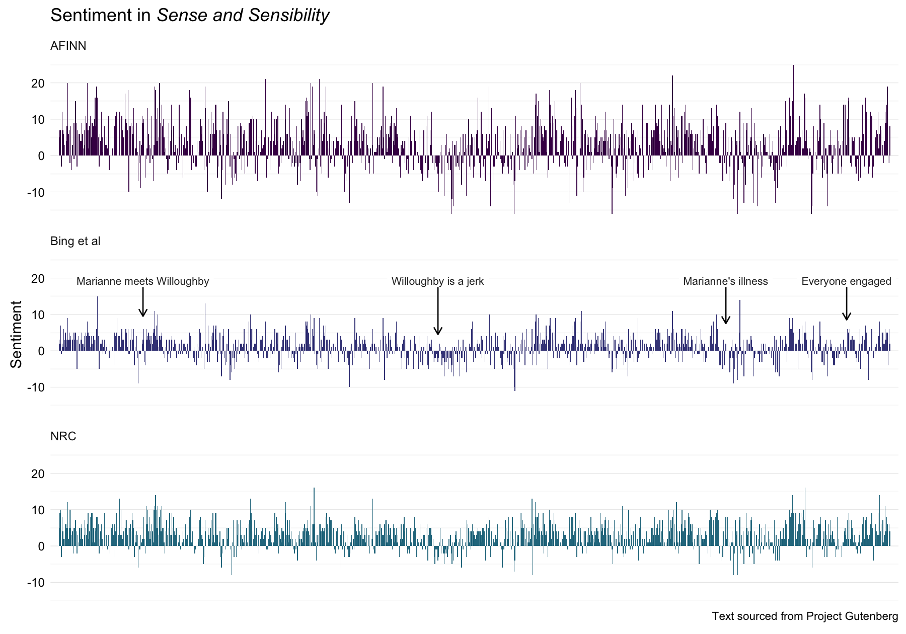
There is another sentiment analysis tool in the Stanford CoreNLP tools, but I have not gotten that one up and running yet (it is written in Java and separate from the R ecosystem). We will stick to the three sentiment tools above; let’s look at sentiment throughout Sense and Sensibility as measured with these three.
SandS <- rbind(process_sentiment(sensesensibility,"afinn") %>% mutate(method = "AFINN"),
               process_sentiment(sensesensibility,"bing") %>% mutate(method = "Bing et al"),
               process_sentiment(sensesensibility,"nrc") %>% mutate(method = "NRC"))
Now let’s make a data frame for annotating the plot and then plot the three methods for sentiment analysis.
caption <- "Text sourced from Project Gutenberg"
annotatetext <- data.frame(x = c(108, 484, 851, 1005), y = rep(19.3, 4),
                           label = c("Marianne meets Willoughby", "Willoughby is a jerk",
                                     "Marianne's illness", "Everyone engaged"),
                           y1 = rep(17.5, 4), y2 = c(9.5, 4.5, 7.5, 8.5),
                           method = factor(rep("Bing et al", 4),
                                           levels = c("AFINN", "Bing et al", "NRC")))

ggplot(data = SandS, aes(x = linenumber, y = sentiment, fill = method)) +
        geom_bar(stat = "identity") +
        facet_wrap(~method, nrow = 3) +
        theme_minimal() +
        ylab("Sentiment") +
        labs(title = expression(paste("Sentiment in ", italic("Sense and Sensibility"))),
             caption = caption) +
        geom_label(data = annotatetext, aes(x, y, label=label), hjust = 0.5,
                  label.size = 0, size = 3, color="#2b2b2b", inherit.aes = FALSE) +
        geom_segment(data = annotatetext, aes(x = x, y = y1, xend = x, yend = y2),
                     arrow = arrow(length = unit(0.05, "npc")), inherit.aes = FALSE) +
        scale_fill_viridis(end = 0.4, discrete=TRUE) +
        scale_x_discrete(expand=c(0.01,0)) +
        theme(strip.text=element_text(hjust=0)) +
        theme(axis.text.y=element_text(margin=margin(r=-10))) +
        theme(plot.caption=element_text(size=9)) +
        theme(legend.position="none") +
        theme(axis.title.x=element_blank()) +
        theme(axis.ticks.x=element_blank()) +
        theme(axis.text.x=element_blank())
I am using the development version of ggplot2 version, available via Github. Hence the nice easy caption below the plot!
The three different methods of calculating sentiment give results that are different in an absolute sense but have similar relative trajectories through the novel. The AFINN method has the largest absolute values, with high postive and negative values. The method of Bing et al. has lower absolute values and appears to label larger blocks of contiguous positive or negative text. The NRC results are shifted higher relative to the other two, labeling the text more positively, but detects similar relative changes in the text. I found similar differences between the methods when looking at the other Jane Austen novels; the NRC sentiment is high, the AFINN sentiment has a lot of variance, the Bing et al. sentiment appears to find longer stretches of similar text, but all three agree roughly on the overall trends in the sentiment through the story. There may be good reasons for picking one of these sentiment analysis tools over the others, but based on these results let’s use the Bing et al. sentiment method for the rest of this post.
How Much Sooner One Tires of Any Thing Than of a Book
Let’s look at the rest of Jane Austen’s novels. First, let’s define a plotting function to use.
plot_sentiment <- function (mySentiment, myAnnotate) {
        g <- ggplot(data = mySentiment, aes(x = linenumber, y = sentiment)) +
                geom_bar(stat = "identity", color = "midnightblue") +
                geom_label(data = myAnnotate, aes(x, y, label=label), hjust = 0.5,
                          label.size = 0, size = 3, color="#2b2b2b", inherit.aes = FALSE) +
                geom_segment(data = myAnnotate, aes(x = x, y = y1, xend = x, yend = y2),
                             arrow = arrow(length = unit(0.04, "npc")), inherit.aes = FALSE) +
                theme_minimal() +
                labs(y = "Sentiment", caption = "Text sourced from Project Gutenberg") +
                scale_x_discrete(expand=c(0.02,0)) +
                theme(plot.caption=element_text(size=8)) +
                theme(axis.text.y=element_text(margin=margin(r=-10))) +
                theme(axis.title.x=element_blank()) +
                theme(axis.ticks.x=element_blank()) +
                theme(axis.text.x=element_blank())
}
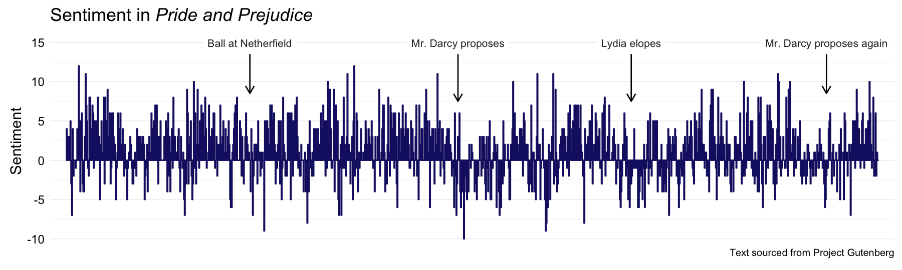
We already spent a good bit of time on Pride and Prejudice last time around, but here it is with the Bing et al. sentiment method.
PP_sentiment <- process_sentiment(prideprejudice, "bing")
PandPannot <- data.frame(x = c(243, 518, 747, 1005), y = rep(14.9, 4),
                           label = c("Ball at Netherfield", "Mr. Darcy proposes",
                                     "Lydia elopes", "Mr. Darcy proposes again"),
                           y1 = rep(13.5, 4), y2 = c(8.5, 7.5, 7.5, 8.5))
p <- plot_sentiment(PP_sentiment, PandPannot)
p + labs(title = expression(paste("Sentiment in ", italic("Pride and Prejudice"))))
Next let’s do Mansfield Park.
MP_sentiment <- process_sentiment(mansfieldpark, "bing")
MPannot <- data.frame(x = c(345, 529, 849, 1224), y = rep(14.9, 4),
                           label = c("Preparing for the play", "Sir Thomas returns",
                                     "Mr. Crawford proposes", "Mr. Crawford's scandal"),
                           y1 = rep(13.5, 4), y2 = c(7.8, 10.2, 8.5, 7.5))
p <- plot_sentiment(MP_sentiment, MPannot)
p + labs(title = expression(paste("Sentiment in ", italic("Mansfield Park"))))
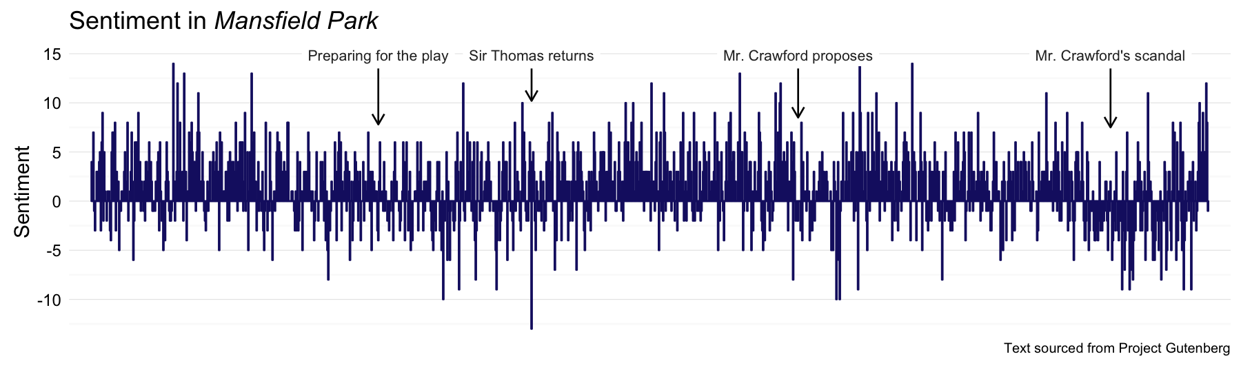
I still feel like Billie Piper was a weird choice for Fanny, but Hayley Atwell as Mary Crawford was GENIUS.
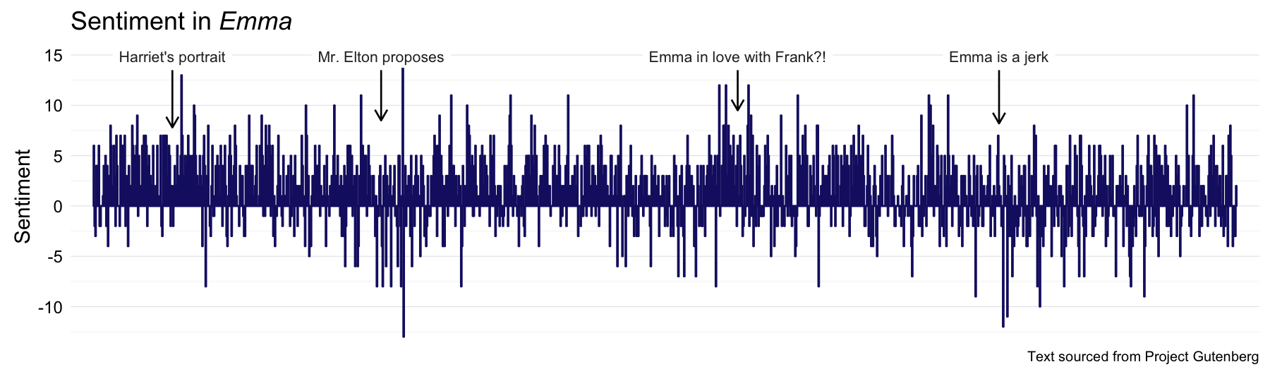
Next up, Emma!
Emma_sentiment <- process_sentiment(emma, "bing")
Emmaannot <- data.frame(x = c(95, 345, 772, 1085), y = rep(14.9, 4),
                           label = c("Harriet's portrait", "Mr. Elton proposes",
                                     "Emma in love with Frank?!", "Emma is a jerk"),
                           y1 = rep(13.5, 4), y2 = c(7.8, 8.5, 9.5, 8.2))
p <- plot_sentiment(Emma_sentiment, Emmaannot)
p + labs(title = expression(paste("Sentiment in ", italic("Emma"))))
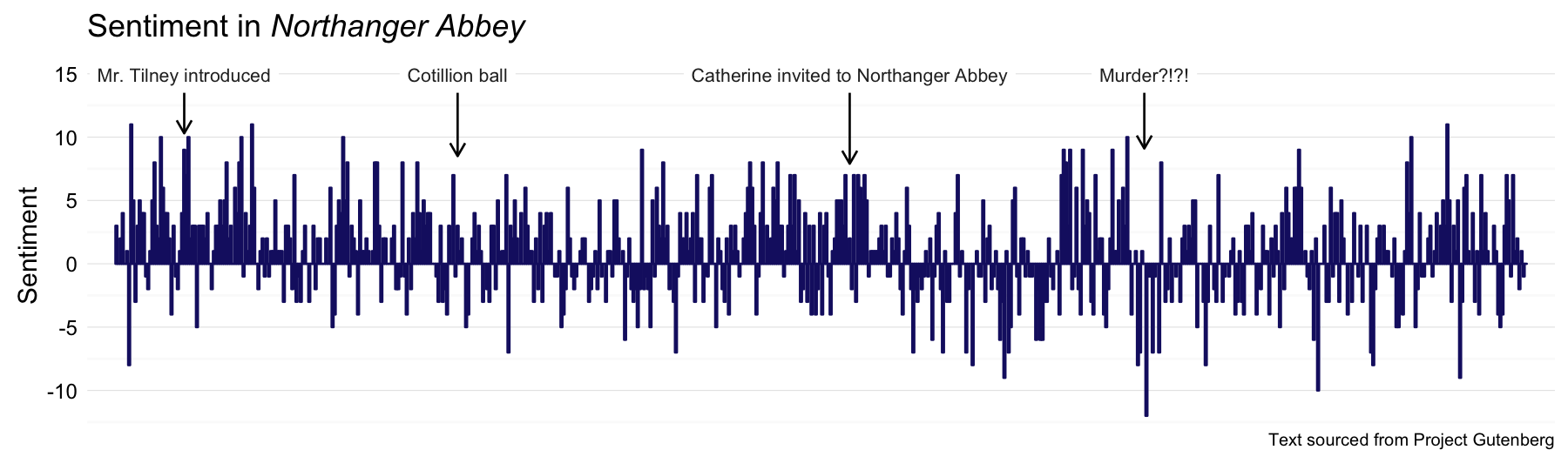
Northanger Abbey was written largely when Austen was quite young, but she revised it later in life and it was published posthumously.
NA_sentiment <- process_sentiment(northangerabbey, "bing")
NAannot <- data.frame(x = c(33, 162, 347, 486), y = rep(14.9, 4),
                           label = c("Mr. Tilney introduced", "Cotillion ball",
                                     "Catherine invited to Northanger Abbey", "Murder?!?!"),
                           y1 = rep(13.5, 4), y2 = c(10.3, 8.5, 7.9, 9.1))
p <- plot_sentiment(NA_sentiment, NAannot)
p + labs(title = expression(paste("Sentiment in ", italic("Northanger Abbey"))))
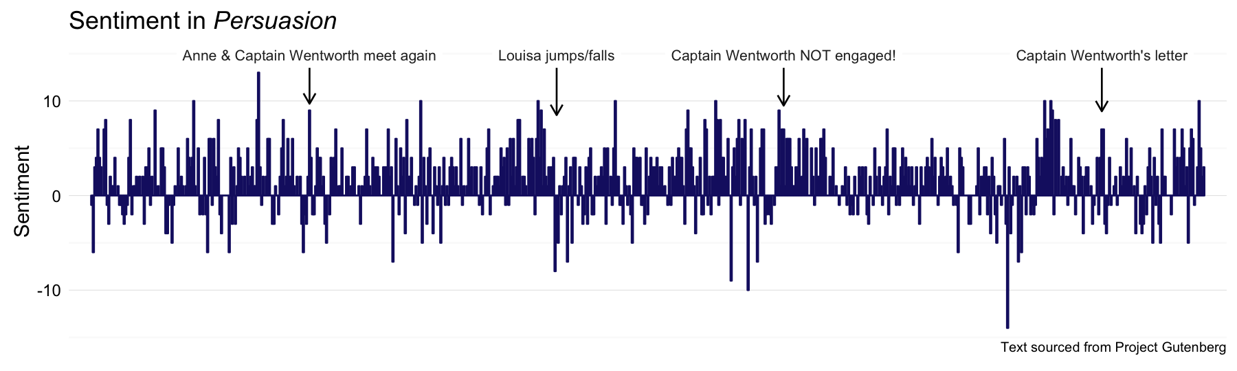
And then there is Austen’s gorgeous final novel, Persuasion.
persuasion_sentiment <- process_sentiment(persuasion, "bing")
Persannot <- data.frame(x = c(142, 302, 449, 655), y = rep(14.9, 4),
                           label = c("Anne & Captain Wentworth meet again", "Louisa jumps/falls",
                                     "Captain Wentworth NOT engaged!", "Captain Wentworth's letter"),
                           y1 = rep(13.5, 4), y2 = c(9.7, 8.5, 9.5, 8.9))
p <- plot_sentiment(persuasion_sentiment, Persannot)
p + labs(title = expression(paste("Sentiment in ", italic("Persuasion"))))
I Am in Half Agony, Half Hope That This Is a Good Idea
Now let’s filter and transform these sentiments using the low-pass Fourier transform. First, let’s get the sentiment for Sense and Sensibility in the same kind of data frame as the rest of the novels.
SS_sentiment <- process_sentiment(sensesensibility, "bing")
Now let’s make a function for finding the transformed values.
fourier_sentiment <- function (sentiment) {
        as.numeric(get_transformed_values(sentiment[,2],
                                          low_pass_size = 3,
                                          scale_vals = TRUE,
                                          scale_range = FALSE))
}
We can now calculate the transformed sentiment plot shapes for all six novels.
plotshape <- rbind(data_frame(linenumber = 1:100, ft = fourier_sentiment(SS_sentiment)) %>%
                           mutate(novel = "Sense and Sensibility"),
      data_frame(linenumber = 1:100, ft = fourier_sentiment(PP_sentiment)) %>%
              mutate(novel = "Pride and Prejudice"),
      data_frame(linenumber = 1:100, ft = fourier_sentiment(MP_sentiment)) %>%
              mutate(novel = "Mansfield Park"),
      data_frame(linenumber = 1:100, ft = fourier_sentiment(Emma_sentiment)) %>%
              mutate(novel = "Emma"),
      data_frame(linenumber = 1:100, ft = fourier_sentiment(NA_sentiment)) %>%
              mutate(novel = "Northanger Abbey"),
      data_frame(linenumber = 1:100, ft = fourier_sentiment(persuasion_sentiment)) %>%
              mutate(novel = "Persuasion"))
plotshape$novel <- factor(plotshape$novel, levels = c("Sense and Sensibility",
                                                      "Pride and Prejudice",
                                                      "Mansfield Park",
                                                      "Emma",
                                                      "Northanger Abbey",
                                                      "Persuasion"))
That’s… maybe not the most elegant way to achieve this step, I admit. Anyway, let’s see what these look like.
ggplot(data = plotshape, aes(x = linenumber, y = ft, fill = novel)) +
        geom_area(alpha = 0.7) +
        facet_wrap(~novel, nrow = 3) +
        theme_minimal() +
        ylab("Transformed Sentiment Value") +
        labs(title = "Sentiment in Jane Austen's Novels",
             caption = caption) +
        scale_fill_viridis(end = 0.4, discrete=TRUE) +
        scale_x_discrete(expand=c(0,0)) +
        theme(strip.text=element_text(hjust=0)) +
        theme(strip.text = element_text(face = "italic")) +
        theme(axis.text.y=element_text(margin=margin(r=-10))) +
        theme(plot.caption=element_text(size=9)) +
        theme(legend.position="none") +
        theme(axis.title.x=element_blank()) +
        theme(axis.ticks.x=element_blank()) +
        theme(axis.text.x=element_blank())
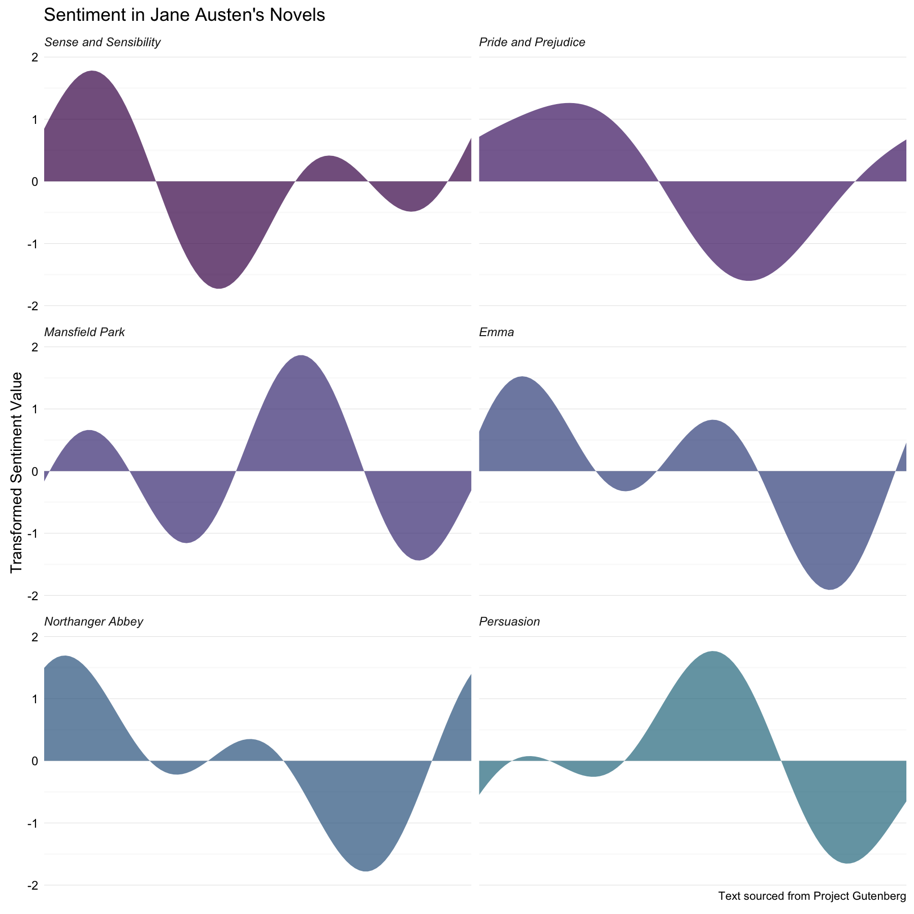
This is super interesting to me. Emma and Northanger Abbey have the most similar plot trajectories, with their tales of immature women who come to understand their own folly and grow up a bit. Mansfield Park and Persuasion also have quite similar shapes, which also is absolutely reasonable; both of these are more serious, darker stories with main characters who are a little melancholic. Persuasion also appears unique in starting out with near-zero sentiment and then moving to more dramatic shifts in plot trajectory; it is a markedly different story from Austen’s other works.
All that said, I have been thinking more about using a Fourier transform in this way and I am not 100% convinced; I think there are some caveats. Making a model of plot shape in this way forces the plot trajectory to be periodic. This doesn’t seem like too much of a problem as far as a general sinusoidal up-and-down pattern, and the shapes do make sense compared to the raw sentiment scores and my human reading of the trajectory of these novels. However, this modeling method forces the plot shape to begin and end at the same sentiment level. Whatever usefulness this method might have, we all have to admit that is a big drawback. It can’t do a good job of modeling any plot shape that has a significantly terrible/wonderful ending compared to its beginning.
The End
It would be nice to think about other options for analyzing or modeling plot shapes beyond this low-pass filter approach. Aside from that, the janeaustenr package is now available and could be used for all sorts of text-y things; network analysis and term frequency (tf-idf) are just a couple of the things I would like to play around with. I am so delighted to be learning about natural language processing. The ideas involved in computational linguistics hit some real sweet spots for me. Heck, if I had known such things were possible ~15 years ago, I may well have gone a whole different direction educationally.
Don’t worry, though, space; you are still my first love.
The R Markdown file used to make this blog post is available [here](https://github.com/juliasilge/juliasilge.github.io/blob/master/_R/2016-03-18-If-I-Loved-NLP-Less.Rmd). I am very happy to hear feedback or questions!