You Must Allow Me To Tell You How Ardently I Admire and Love Natural Language Processing
By Julia Silge
March 8, 2016
It is a truth universally acknowledged that sentiment analysis is super fun, and Pride and Prejudice is probably my very favorite book in all of literature, so let’s do some Jane Austen natural language processing.
Project Gutenberg makes e-texts available for many, many books, including Pride and Prejudice which is available here. I am using the plain text UTF-8 file available at that link for this analysis. Let’s read the file and get it ready for analysis.
Munge the Data, But ELEGANTLY, As Would Befit Jane Austen
The plain text file has lines that are just over 70 characters long. We can read them in using the readr library, which is super fast and easy to use. Let’s use the skip and n_max options to leave out the Project Gutenberg header and footer information and just get the actual text of the novel. Lines of 70 characters are not really a big enough chunk of text to be useful for my purposes here (that’s not even a tweet!) so let’s use stringr to concatenate these lines in chunks of 10. That gives us sort of paragraph-sized chunks of text.
library(readr)
library(stringr)
rawPandP <- read_lines("./pg1342.txt", skip = 30, n_max = 13032)
PandP <- character()
for (i in seq_along(rawPandP)) {
        if (i%%10 == 1) PandP[ceiling(i/10)] <- str_c(rawPandP[i],
                                                     rawPandP[i+1],
                                                     rawPandP[i+2],
                                                     rawPandP[i+3],
                                                     rawPandP[i+4],
                                                     rawPandP[i+5],
                                                     rawPandP[i+6],
                                                     rawPandP[i+7],
                                                     rawPandP[i+8],
                                                     rawPandP[i+9], sep = " ")
}
Maybe you don’t think for loops are elegant, actually, but I could not come up with a way to vectorize this.
Mr. Darcy Delivered His Sentiments in a Manner Little Suited to Recommend Them
To do the sentiment analysis, let’s use the
NRC Word-Emotion Association Lexicon of Saif Mohammad and Peter Turney. You can read a bit more about the NRC sentiment dictionary and how it is used in
one of my previous blog posts. It is implemented in R in the syuzhet package.
I was not sure, when I stopped to think about it, exactly how appropriate this tool is for analyzing 200-year-old text. Language changes over time and from what I can tell, the NRC lexicon is designed and validated to measure the sentiment in contemporary English. It was created via crowdsourcing on Amazon’s Mechanical Turk. However, it doesn’t seem to do badly on Jane Austen’s prose; the sentiment results are about what one would expect compared to a human reading of the meaning. If anything, the text in Pride and Prejudice involves more dramatic vocabulary than a lot of contemporary English prose and it is easier for a tool like the NRC dictionary to pick up on the emotions involved.
Let’s look at some examples.
library(syuzhet)
get_nrc_sentiment("Nobody can tell what I suffer! But it is always so. Those who do not complain are never pitied.")
##   anger anticipation disgust fear joy sadness surprise trust negative positive
## 1     1            0       0    0   0       1        0     0        2        0
Oh, Mrs. Bennett…
get_nrc_sentiment("And your defect is to hate everybody.")
##   anger anticipation disgust fear joy sadness surprise trust negative positive
## 1     2            0       1    1   0       1        0     0        2        0
get_nrc_sentiment("You must allow me to tell you how ardently I admire and love you.")
##   anger anticipation disgust fear joy sadness surprise trust negative positive
## 1     0            0       0    0   1       0        0     1        0        2
So let’s start from a working hypothesis that the NRC lexicon can be applied to this novel and do the sentiment analysis for each chunk of text in our dataframe. At the same time, let’s make a linenumber that counts up through the novel.
PandPnrc <- cbind(linenumber = seq_along(PandP), get_nrc_sentiment(PandP))
Dividing Up the Volumes
Pride and Prejudice contains 61 chapters divided into three volumes; Volume I is Chapters 1-23, Volume II is Chapters 24-42, and Volume III is Chapters 43-61. Let’s find where these breaks between volumes have ended up.
grep("Chapter 1 ", PandP)
## [1] 1
grep("Chapter 24", PandP)
## [1] 451
grep("Chapter 43", PandP)
## [1] 805
Let’s make a volume factor for the dataframe and then restart the linenumber count at the beginning of each volume.
PandPnrc$volume <- "Volume I"
PandPnrc[grep("Chapter 24", PandP):length(PandP),'volume'] <- "Volume II"
PandPnrc[grep("Chapter 43", PandP):length(PandP),'volume'] <- "Volume III"
PandPnrc$volume <- as.factor(PandPnrc$volume)
PandPnrc$linenumber[PandPnrc$volume == "Volume II"] <- seq_along(PandP)
PandPnrc$linenumber[PandPnrc$volume == "Volume III"] <- seq_along(PandP)
Positive and Negative Sentiment
First let’s look at the overall postive vs. negative sentiment in the text of Pride and Prejudice before looking at more specific emotions.
library(dplyr)
library(reshape2)
PandPnrc$negative <- -PandPnrc$negative
posneg <- PandPnrc %>% select(linenumber, volume, positive, negative) %>%
        melt(id = c("linenumber", "volume"))
names(posneg) <- c("linenumber", "volume", "sentiment", "value")
Here, each chunk of text has a score for the positive sentiment and the negative sentiment; a given chunk of text could have high scores for both, low scores for both, or any combination thereof. I have made the sign of the negative sentiment negative for plotting purposes. Let’s make a dataframe of some important events in the novel to annotate the plots; I found the chapters for these events and matched them up to the correct volumes and line numbers.
annotatetext <- data.frame(x = c(114, 211, 307, 183, 91, 415), y = rep(18.3, 6),
                           label = c("Jane's illness", "Mr. Collins arrives",
                                     "Ball at Netherfield", "Mr. Darcy proposes",
                                     "Lydia elopes", "Mr. Darcy proposes again"),
                           volume = factor(c("Volume I", "Volume I",
                                             "Volume I", "Volume II",
                                             "Volume III", "Volume III"),
                                           levels = c("Volume I", "Volume II", "Volume III")))
annotatearrow <- data.frame(x = c(114, 211, 307, 183, 91, 415),
                            y1 = rep(17, 6), y2 = c(11.2, 10.7, 11.4, 13.5, 10.5, 11.5),
                            volume = factor(c("Volume I", "Volume I",
                                              "Volume I", "Volume II",
                                              "Volume III", "Volume III"),
                                            levels = c("Volume I", "Volume II", "Volume III")))
Now let’s plot the positive and negative sentiment.
library(ggplot2)
library(ggthemes)
ggplot(data = posneg, aes(x = linenumber, y = value, color = sentiment)) +
        facet_wrap(~volume, nrow = 3) +
        geom_point(size = 4, alpha = 0.5) + theme_minimal() +
        ylab("Sentiment") +
        ggtitle(expression(paste("Positive and Negative Sentiment in ",
                                 italic("Pride and Prejudice")))) +
        theme(legend.title=element_blank()) +
        theme(axis.title.x=element_blank()) +
        theme(axis.ticks.x=element_blank()) +
        theme(axis.text.x=element_blank()) +
        geom_text(data = annotatetext, aes(x,y,label=label), hjust = 0.5,
                  size = 3, inherit.aes = FALSE) +
        geom_segment(data = annotatearrow, aes(x = x, y = y1, xend = x, yend = y2),
                     arrow = arrow(length = unit(0.05, "npc")), inherit.aes = FALSE) +
        theme(legend.justification=c(1,1), legend.position=c(1, 0.71)) +
        scale_color_manual(values = c("aquamarine3", "midnightblue"))
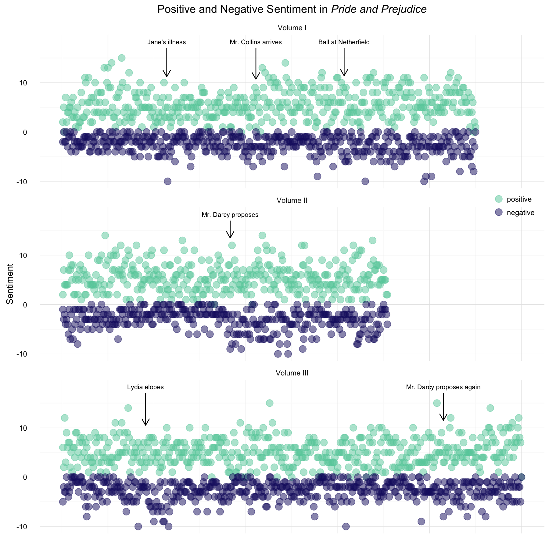
Narrative time runs along the x-axis. Volume II is the shortest of the three parts of the novel. We can see here that the positive sentiment scores are overall much higher than the negative sentiment, which makes sense for Jane Austen’s writing style. We can see some more strongly negative sentiment when Mr. Darcy proposes for the first time and when Lydia elopes. Let’s try visualizing these same data with a bar chart instead of points.
ggplot(data = posneg, aes(x = linenumber, y = value, color = sentiment, fill = sentiment)) +
        facet_wrap(~volume, nrow = 3) +
        geom_bar(stat = "identity", position = "dodge") + theme_minimal() +
        ylab("Sentiment") +
        ggtitle(expression(paste("Positive and Negative Sentiment in ",
                                 italic("Pride and Prejudice")))) +
        theme(legend.title=element_blank()) +
        theme(axis.title.x=element_blank()) +
        theme(axis.ticks.x=element_blank()) +
        theme(axis.text.x=element_blank()) +
        theme(legend.justification=c(1,1), legend.position=c(1, 0.71)) +
        geom_text(data = annotatetext, aes(x,y,label=label), hjust = 0.5,
                  size = 3, inherit.aes = FALSE) +
        geom_segment(data = annotatearrow, aes(x = x, y = y1, xend = x, yend = y2),
                     arrow = arrow(length = unit(0.05, "npc")), inherit.aes = FALSE) +
        scale_fill_manual(values = c("aquamarine3", "midnightblue")) +
        scale_color_manual(values = c("aquamarine3", "midnightblue"))
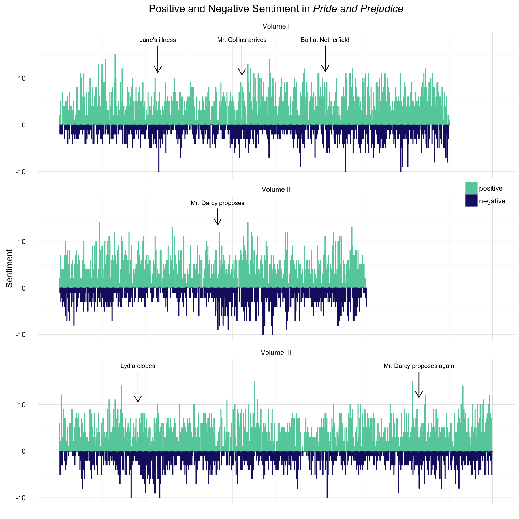
I like certain aspects of both of these styles of plots. What do you think? Is one of these clearer or more appealing to you?
Fourier Transform Time
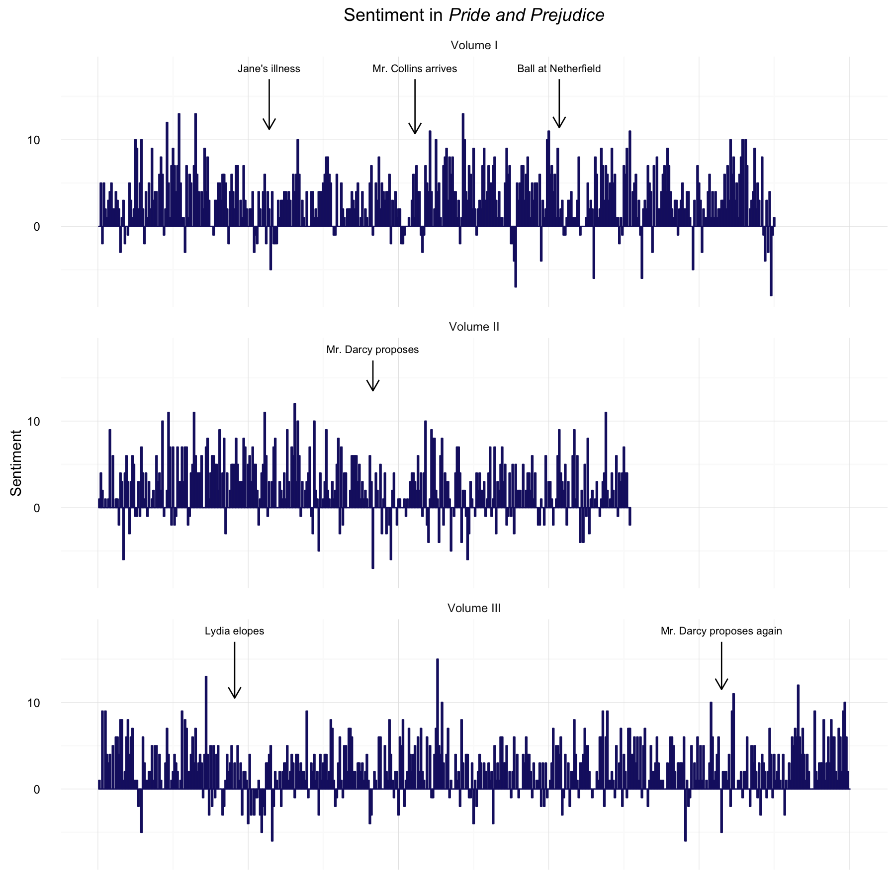
The previous plots showed both the positive and negative sentiment, but we could also take each chunk of text and assign one value, the positive sentiment minus the negative sentiment for an overall sense of the emotional content of the text. Let’s do that for a new view of the novel’s content.
PandPsentiment <- data.frame(cbind(linenumber = seq_along(PandP),
                                   sentiment = get_sentiment(PandP, method = "nrc")))
PandPsentiment$volume <- "Volume I"
PandPsentiment[grep("Chapter 24", PandP):length(PandP),'volume'] <- "Volume II"
PandPsentiment[grep("Chapter 43", PandP):length(PandP),'volume'] <- "Volume III"
PandPsentiment$volume <- as.factor(PandPsentiment$volume)
PandPsentiment$linenumber[PandPsentiment$volume == "Volume II"] <- seq_along(PandP)
PandPsentiment$linenumber[PandPsentiment$volume == "Volume III"] <- seq_along(PandP)
Now let’s plot this single measure of the sentiment in the novel.
ggplot(data = PandPsentiment, aes(x = linenumber, y = sentiment)) +
        facet_wrap(~volume, nrow = 3) +
        geom_bar(stat = "identity", position = "dodge", color = "midnightblue") +
        theme_minimal() +
        ylab("Sentiment") +
        ggtitle(expression(paste("Sentiment in ", italic("Pride and Prejudice")))) +
        theme(axis.title.x=element_blank()) +
        theme(axis.ticks.x=element_blank()) +
        theme(axis.text.x=element_blank()) +
        theme(legend.justification=c(1,1), legend.position=c(1, 0.71)) +
        geom_text(data = annotatetext, aes(x,y,label=label), hjust = 0.5,
                  size = 3, inherit.aes = FALSE) +
        geom_segment(data = annotatearrow, aes(x = x, y = y1, xend = x, yend = y2),
                     arrow = arrow(length = unit(0.05, "npc")), inherit.aes = FALSE)
To better see the overall trajectory of the narrative, we can filter and transform these sentiment scores using a low-pass filter Fourier transform. Matthew Jockers, the author of the syuzhet package, describes this
in more detail here.
PandPft <- as.numeric(get_transformed_values(PandPsentiment$sentiment,
                                  low_pass_size = 3,
                                  scale_vals = TRUE,
                                  scale_range = FALSE))
PandPft <- data.frame(cbind(linenumber = seq_along(PandPft), ft = PandPft))
Now, I am a little rusty on the Fourier transform. I haven’t thought much about it since I was a physics undergrad taking an electronics lab; I vaguely remember that I made a square wave by adding up a bunch of sine waves. In the case here with text from a novel, the sentiment scores are the time domain signal. Taking the Fourier transform finds the set of sinusoidal functions to sum up to represent the time domain signal. Thus, the Fourier transform shows us where the narrative sentiment is positive/negative, and the low-pass filter allows us to see the overall structure in the narrative (i.e. low frequency structure) while filtering out high frequency information. We would just have to decide how many components to keep for the low-pass filtering.
ggplot(data = PandPft, aes(x = linenumber, y = ft)) +
        geom_bar(stat = "identity", alpha = 0.8, color = "midnightblue", fill = "midnightblue") +
        theme_minimal() +
        ylab("Transformed Sentiment Value") +
        ggtitle(expression(paste("Sentiment in ", italic("Pride and Prejudice")))) +
        theme(axis.title.x=element_blank()) +
        theme(axis.ticks.x=element_blank()) +
        theme(axis.text.x=element_blank()) +
        annotate("text", size = 3, x = c(9, 23, 49, 69, 94),
                 y = c(-0.2, -0.5, 0.5, 0.2, 0.7),
                 label = c("Jane's illness", "Ball at Netherfield",
                           "Mr. Darcy proposes", "Lydia elopes",
                           "Mr. Darcy proposes again")) +
        annotate("segment", arrow = arrow(length = unit(0.03, "npc")),
                 x = c(9, 23, 49, 69, 94), xend = c(9, 23, 49, 69, 94),
                 y = c(-0.16, -0.46, 0.44, 0.15, 0.64),
                 yend = c(-0.02, -0.02 , 0.02, 0.02, 0.2))
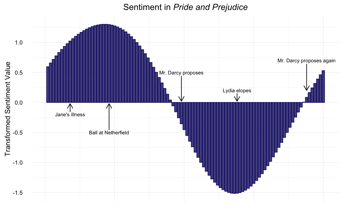
This probably jumps out as pretty obvious, but the values have been scaled and centered here to show the narrative shape. The raw sentiment scores were all mostly positive in Pride and Prejudice but the filtered and transformed sentiment scores have been scaled and centered to visualize the overall structure of the narrative. Notice the important events that correspond to the max/min in the transformed and filtered sentiment score. I am just delighted about that. Math! It is the best. I do want to be careful not to overemphasize that result just now, though, because it depends on how many Fourier components we keep during the low-pass filtering. This plot is made by keeping 3 components, the default in the syuzhet package; the shape will look a little different with more small-scale (i.e., higher frequency) structure if we keep 4 or 5 components and the important plot events may not align quite as perfectly with a maximum, for example. I would like to explore this point more.
The FEEEEEEEEEEELINGS
The NRC lexicon includes scores for eight emotions, along with the overall positive and negative sentiment scores. Let’s see how these emotion scores change during the novel. We will need bigger chunks of text to make reasonable looking plots, so let’s go back and concatenate our chunks into bits that are five times larger. (The last chunk will be a bit shorter because it doesn’t come out exactly even.)
PandP[1304] <- ""
PandP[1305] <- ""
shorterPandP <- character()
for (i in seq_along(PandP)) {
        if (i%%5 == 1) shorterPandP[ceiling(i/5)] <- str_c(PandP[i],
                                                      PandP[i+1],
                                                      PandP[i+2],
                                                      PandP[i+3],
                                                      PandP[i+4], sep = " ")
}
Now let’s find the sentiment scores, divide between the three volumes of the novel, and melt for plotting.
PandPnrc <- cbind(linenumber = seq_along(shorterPandP), get_nrc_sentiment(shorterPandP))
PandPnrc$volume <- "Volume I"
PandPnrc[grep("Chapter 24", shorterPandP):length(shorterPandP),'volume'] <- "Volume II"
PandPnrc[grep("Chapter 43", shorterPandP):length(shorterPandP),'volume'] <- "Volume III"
PandPnrc$volume <- as.factor(PandPnrc$volume)
PandPnrc$linenumber[PandPnrc$volume == "Volume II"] <- seq_along(shorterPandP)
PandPnrc$linenumber[PandPnrc$volume == "Volume III"] <- seq_along(shorterPandP)
emotions <- PandPnrc %>% select(linenumber, volume, anger, anticipation,
                                      disgust, fear, joy, sadness, surprise,
                                      trust) %>%
        melt(id = c("linenumber", "volume"))
names(emotions) <- c("linenumber", "volume", "sentiment", "value")
Let’s capitalize the names of the emotions for plotting, and also let’s reorder the factor so that more postive emotions are together in the plot and more negative emotions are together in the plot.
levels(emotions$sentiment) <- c("Anger", "Anticipation", "Disgust", "Fear",
                                "Joy", "Sadness", "Surprise", "Trust")
emotions$sentiment = factor(emotions$sentiment,levels(emotions$sentiment)[c(5,8,2,7,6,3,4,1)])
For plotting the emotions, let’s make heat maps in the style of Bob Rudis. When I saw him put some examples of these heat maps on Twitter, I just knew that I needed to make some.
library(viridis)
ggplot(data = emotions, aes(x = linenumber, y = sentiment, fill = value)) +
        geom_tile(color="white", size=0.1) +
        facet_wrap(~volume, nrow = 3) +
        scale_fill_viridis(name="Sentiment\nScore") +
        coord_equal() + theme_tufte(base_family="Helvetica") +
        labs(x=NULL, y=NULL,
             title=expression(paste("Sentiment in ", italic("Pride and Prejudice")))) +
        theme(axis.ticks=element_blank(), axis.text.x=element_blank()) +
        scale_x_discrete(expand=c(0,0)) +
        theme(axis.text=element_text(size=6)) +
        theme(panel.border=element_blank()) +
        theme(legend.title=element_text(size=6)) +
        theme(legend.title.align=1) +
        theme(legend.text=element_text(size=6)) +
        theme(legend.position="bottom") +
        theme(legend.key.size=unit(0.2, "cm")) +
        theme(legend.key.width=unit(1, "cm"))
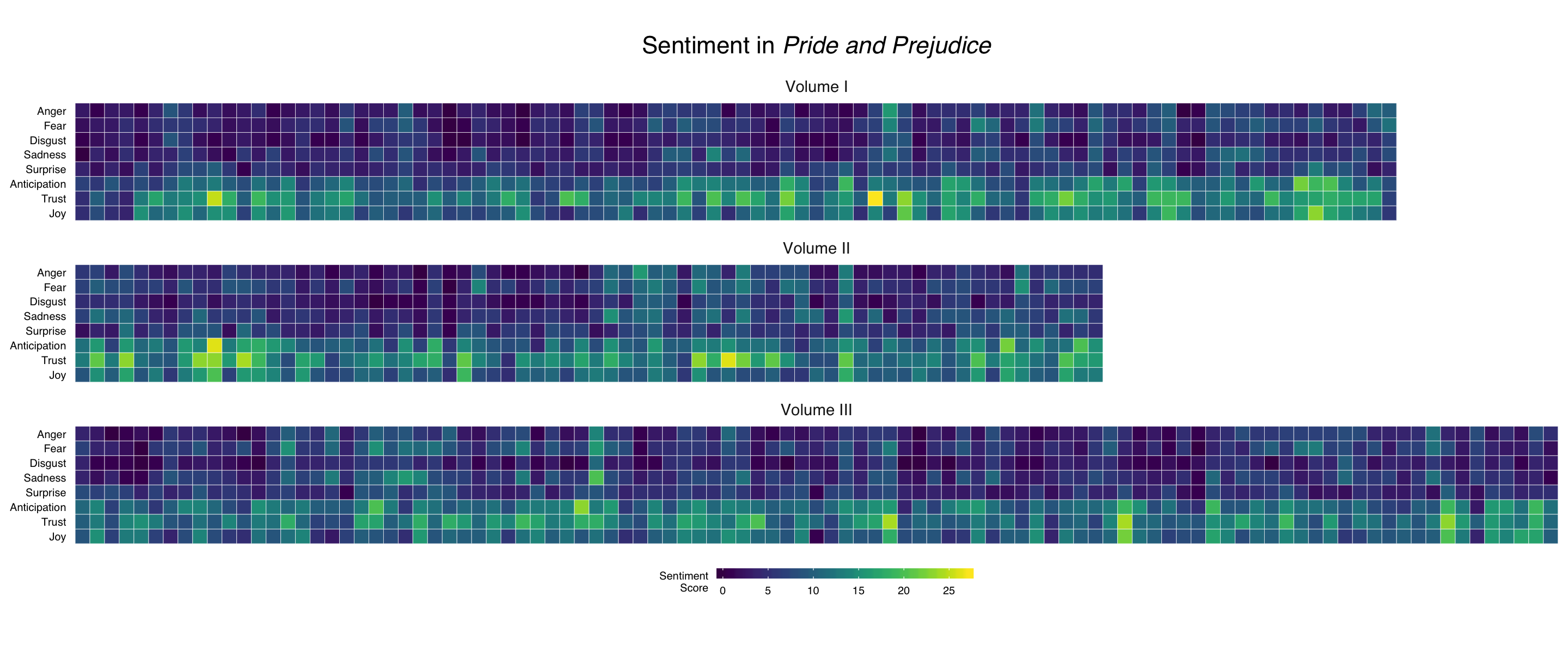
Oh, they’re so pretty… We can see the positive emotions are stronger than the negative ones, which is sensible given Austen’s bright, humorous writing style. The negative emotions are stronger in the middle of Volume II when Mr. Darcy proposes for the first time and near the beginning of Volume III when Lydia elopes.
The End
Wow, this was so much fun, although obviously I have outed myself as a super fan. Good thing I have no shame about that whatsoever. The Fourier transformed sentiment values were so interesting, and are perfect for comparing across different texts. I am eager to try that out on some different novels. Boy, I just love that we can do MATH on WORDS; those are two of my very favorite things. The R Markdown file used to make this blog post is available here. I am very happy to hear feedback or questions!