Where are #TidyTuesday haunted cemeteries compared to haunted schools?

This is the latest in my series of screencasts! It’s spooky season, and this screencast focuses on how to compute weighted log odds using this week’s #TidyTuesday dataset on haunted places in the United States. 👻

Here is the code I used in the video, for those who prefer reading instead of or in addition to video.

Explore data

Our analysis goal here is to understand how different types of haunted places in the United States vary by state. Let’s start by reading in the data:

library(tidyverse)
haunted_places <- read_csv('https://raw.githubusercontent.com/rfordatascience/tidytuesday/master/data/2023/2023-10-10/haunted_places.csv')

The description variable is longer text explaining details about the haunting, while the location variable is shorter text describing the haunted location. Which states are these hauntings in?

haunted_places |> 
  count(state, sort = TRUE)

# A tibble: 51 × 2
   state             n
   <chr>         <int>
 1 California     1070
 2 Texas           696
 3 Pennsylvania    649
 4 Michigan        529
 5 Ohio            477
 6 New York        459
 7 Illinois        395
 8 Kentucky        370
 9 Indiana         351
10 Massachusetts   342
# ℹ 41 more rows

And what kinds of places are haunted?

haunted_places |> 
  slice_sample(n = 10) |> 
  select(location)

# A tibble: 10 × 1
   location                  
   <chr>                     
 1 Single T Canal            
 2 Hwy521                    
 3 Santaquin Canyon          
 4 Syracuse Cemetery         
 5 Del Frisco's Steakhouse   
 6 Walt Disney World         
 7 the Tanning Yards         
 8 Moonshadows Restaurant    
 9 Refugio County Court House
10 The Legend of Big Liz     

What are the most common words used for the haunted locations?

library(tidytext)

haunted_places |> 
  unnest_tokens(word, location) |> 
  count(word, sort = TRUE)

# A tibble: 7,765 × 2
   word           n
   <chr>      <int>
 1 school      1217
 2 the          989
 3 cemetery     751
 4 high         700
 5 old          599
 6 house        502
 7 university   500
 8 road         437
 9 of           406
10 college      373
# ℹ 7,755 more rows

Looks like there are lots of haunted cemeteries, which seems reasonable to me, but also lots of haunted schools! 😱 Haunted schools??!? Won’t someone think of the children? I don’t approve at all.

Weighted log odds

I’d like to know what states are more likely to have haunted cemeteries and what states are more likely to have haunted schools, so I can know which states keep their hauntings where they belong. Let’s use tidylo, a package for weighted log odds using tidy data principles. A log odds ratio is a way of expressing probabilities, and we can weight a log odds ratio so that our implementation does a better job dealing with different features having different counts. Think about how the different states have different numbers of haunted places; we’d like to compute a log odds ratio that gives us a more robust estimate across the states with many haunted places and those with few. You can read more about tidylo in a previous blog post.

To start, let’s create a dataset of counts:

haunted_counts <-
  haunted_places |> 
  mutate(location = str_to_lower(location)) |> 
  mutate(location = case_when(
    str_detect(location, "cemetery|graveyard") ~ "cemetery",
    str_detect(location, "school") ~ "school",
    .default = "other"
  )) |> 
  count(state_abbrev, location)

haunted_counts

# A tibble: 149 × 3
   state_abbrev location     n
   <chr>        <chr>    <int>
 1 AK           cemetery     4
 2 AK           other       23
 3 AK           school       5
 4 AL           cemetery    19
 5 AL           other      187
 6 AL           school      18
 7 AR           cemetery    16
 8 AR           other       91
 9 AR           school      12
10 AZ           cemetery     3
# ℹ 139 more rows

Now we can compute the log odds, weighted (the tidylo default) via empirical Bayes:

library(tidylo)

haunted_counts |> 
  bind_log_odds(location, state_abbrev, n) |> 
  group_by(location) |> 
  slice_max(log_odds_weighted, n = 5) |> 
  mutate(state_abbrev = reorder(state_abbrev, log_odds_weighted)) |> 
  ggplot(aes(log_odds_weighted, state_abbrev, fill = location)) +
  geom_col(show.legend = FALSE) +
  facet_wrap(vars(location), scales = "free") +
  scale_fill_brewer(palette = "Dark2") +
  labs(x = "Weighted log odds (empirical Bayes)", y = NULL)

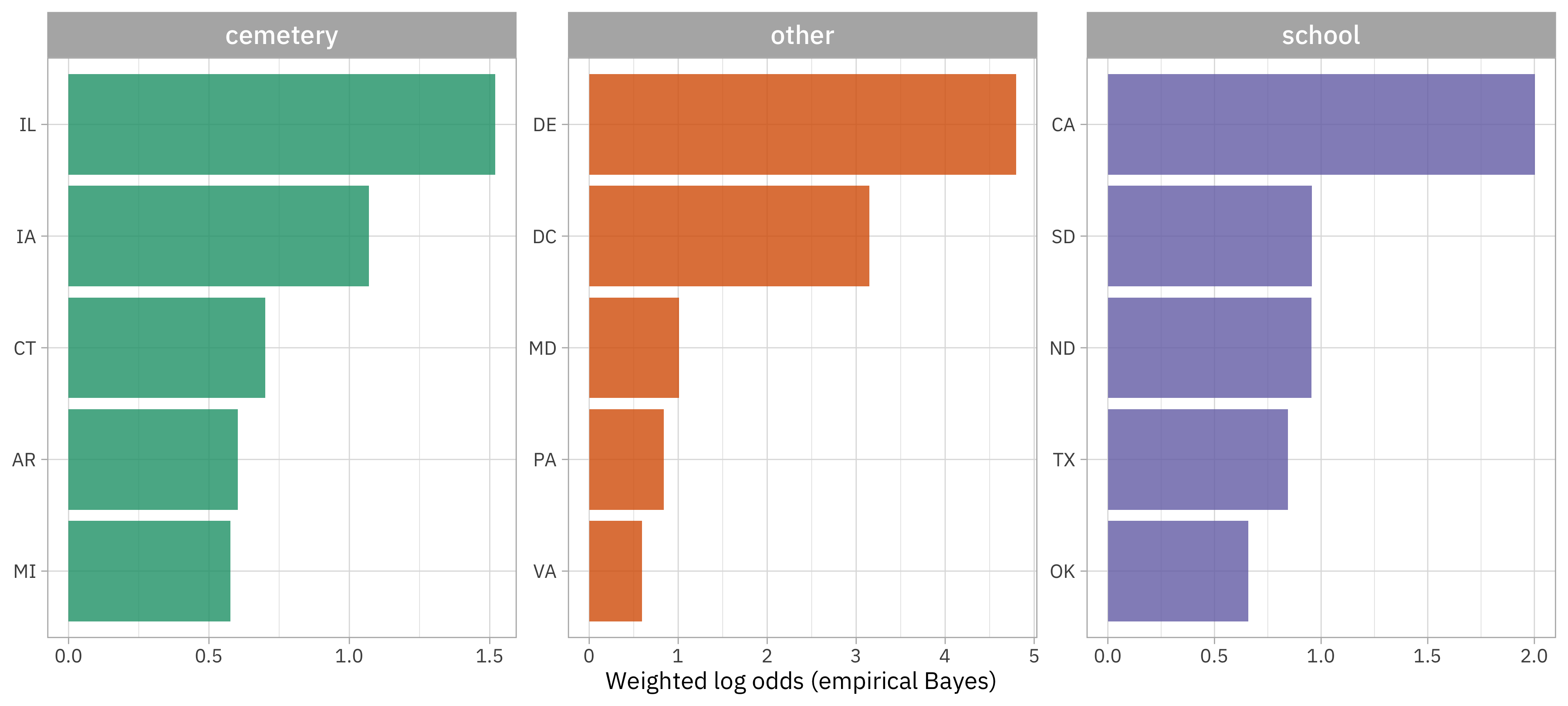
This plot shows us that:

• Illinois, Idaho, and Connecticut are reasonable places where haunted locations are more likely to be cemeteries compared to other states.
• The haunting situation in California, South Dakota, and North Dakota is not good as their haunted locations are more likely to be schools. Beware! 👻
• Delaware, Washington DC, and Maryland have haunted locations that are more likely to be something other than cemeteries and schools, compared to the other states. What are some of these, specifically in DC?

haunted_places |> 
  filter(state_abbrev == "DC") |> 
  slice_sample(n = 10) |> 
  select(location)

# A tibble: 10 × 1
   location        
   <chr>           
 1 White House     
 2 White House     
 3 Trinity College 
 4 Capitol Building
 5 Fort McNair     
 6 White House     
 7 White House     
 8 The Hay         
 9 Capitol building
10 Georgetown      

Seems like the White House is pretty haunted!