How often does Roy Kent say "F*CK"?

This is the latest in my series of screencasts! This screencast focuses on how to compute bootstrap confidence intervals, using this week’s #TidyTuesday dataset on Roy Kent’s colorful language. 🤬

Here is the code I used in the video, for those who prefer reading instead of or in addition to video.

Explore data

It’s hard not to love the show Ted Lasso or one of its most compelling characters, Roy Kent, and our modeling goal here is to estimate how his use of what appears to be his favorite word depends on his coaching status and/or his dating status. This dataset was created by Deepsha Menghani for her excellent talk at posit::conf(2023), and you should definitely keep an eye out for the video when it becomes available later this year. Let’s start by reading in the data:

library(tidyverse)
library(richmondway)
data(richmondway)
glimpse(richmondway)

## Rows: 34
## Columns: 16
## $ Character         <chr> "Roy Kent", "Roy Kent", "Roy Kent", "Roy Kent", "Roy…
## $ Episode_order     <dbl> 1, 2, 3, 4, 5, 6, 7, 8, 9, 10, 11, 12, 13, 14, 15, 1…
## $ Season            <dbl> 1, 1, 1, 1, 1, 1, 1, 1, 1, 1, 2, 2, 2, 2, 2, 2, 2, 2…
## $ Episode           <dbl> 1, 2, 3, 4, 5, 6, 7, 8, 9, 10, 1, 2, 3, 4, 5, 6, 7, …
## $ Season_Episode    <chr> "S1_e1", "S1_e2", "S1_e3", "S1_e4", "S1_e5", "S1_e6"…
## $ F_count_RK        <dbl> 2, 2, 7, 8, 4, 2, 5, 7, 14, 5, 11, 10, 2, 2, 23, 12,…
## $ F_count_total     <dbl> 13, 8, 13, 17, 13, 9, 15, 18, 22, 22, 16, 22, 8, 6, …
## $ cum_rk_season     <dbl> 2, 4, 11, 19, 23, 25, 30, 37, 51, 56, 11, 21, 23, 25…
## $ cum_total_season  <dbl> 13, 21, 34, 51, 64, 73, 88, 106, 128, 150, 16, 38, 4…
## $ cum_rk_overall    <dbl> 2, 4, 11, 19, 23, 25, 30, 37, 51, 56, 67, 77, 79, 81…
## $ cum_total_overall <dbl> 13, 21, 34, 51, 64, 73, 88, 106, 128, 150, 166, 188,…
## $ F_score           <dbl> 0.1538462, 0.2500000, 0.5384615, 0.4705882, 0.307692…
## $ F_perc            <dbl> 15.4, 25.0, 53.8, 47.1, 30.8, 22.2, 33.3, 38.9, 63.6…
## $ Dating_flag       <chr> "No", "No", "No", "No", "No", "No", "No", "Yes", "Ye…
## $ Coaching_flag     <chr> "No", "No", "No", "No", "No", "No", "No", "No", "No"…
## $ Imdb_rating       <dbl> 7.8, 8.1, 8.5, 8.2, 8.9, 8.5, 9.0, 8.7, 8.6, 9.1, 7.…

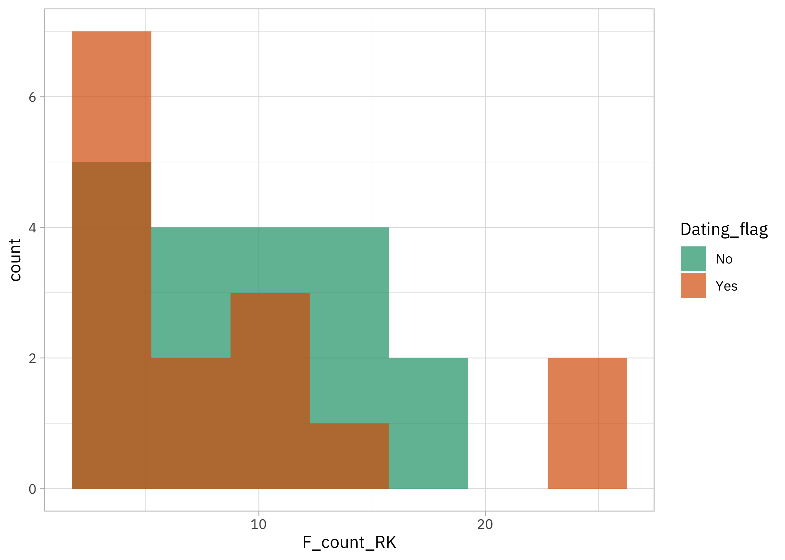
This is not what you call a large dataset but we can check out the distribution of how often Roy Kent says “f*ck” per episode. Can we compare when he is dating Keeley vs. not?

richmondway |> 
    ggplot(aes(F_count_RK, fill = Dating_flag)) +
    geom_histogram(position = "identity", bins = 7, alpha = 0.7) +
    scale_fill_brewer(palette = "Dark2")

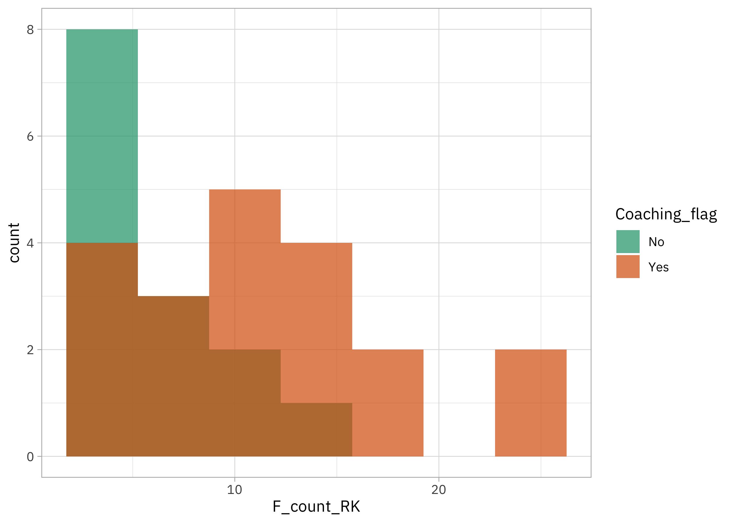
Or what about when he coaching vs. not?

richmondway |> 
    ggplot(aes(F_count_RK, fill = Coaching_flag)) +
    geom_histogram(position = "identity", bins = 7, alpha = 0.7) +
    scale_fill_brewer(palette = "Dark2")

It looks like maybe there are differences here but it’s a small dataset, so let’s use statistical modeling to help us be more sure what we are seeing.

Bootstrap confidence intervals for Poisson regression

There isn’t much code in what we’re about to do, but let’s outline two important pieces of what is going on:

• These are counts of Roy Kent’s F-bombs per episode, so we want to use a model that is a good fit for count data, i.e. Poisson regression.
• We could fit a Poisson regression model one time to this dataset, but it’s such a tiny dataset that we might not have much confidence in the results. Instead, we want to use bootstrap resamples to fit our model a whole bunch of times to get confidence intervals, and then use these replicate results to estimate the impact of coaching and dating.

We can use the reg_intervals() function from rsample to do this all at once. If we use keep_reps = TRUE, we will get each individual model result in our results:

library(rsample)

set.seed(123)
poisson_intervals <- 
    reg_intervals(
        F_count_RK ~ Dating_flag + Coaching_flag, 
        data = richmondway, 
        model_fn = "glm", 
        family = "poisson",
        keep_reps = TRUE
    )

poisson_intervals

## # A tibble: 2 × 7
##   term             .lower .estimate .upper .alpha .method          .replicates
##   <chr>             <dbl>     <dbl>  <dbl>  <dbl> <chr>     <list<tibble[,2]>>
## 1 Coaching_flagYes  0.236    0.654   1.04    0.05 student-t        [1,001 × 2]
## 2 Dating_flagYes   -0.351    0.0428  0.448   0.05 student-t        [1,001 × 2]

Notice the .replicates column where we have each of the 1000 results from our 1000 bootstrap resamples. We can unnest() this column and make a visualization:

poisson_intervals |>
    mutate(term = str_remove(term, "_flagYes")) |> 
    unnest(.replicates) |>
    ggplot(aes(estimate, fill = term)) +
    geom_vline(xintercept = 0, linewidth = 1.5, lty = 2, color = "gray50") +
    geom_histogram(alpha = 0.8, show.legend = FALSE) +
    facet_wrap(vars(term)) +
    scale_fill_brewer(palette = "Accent")

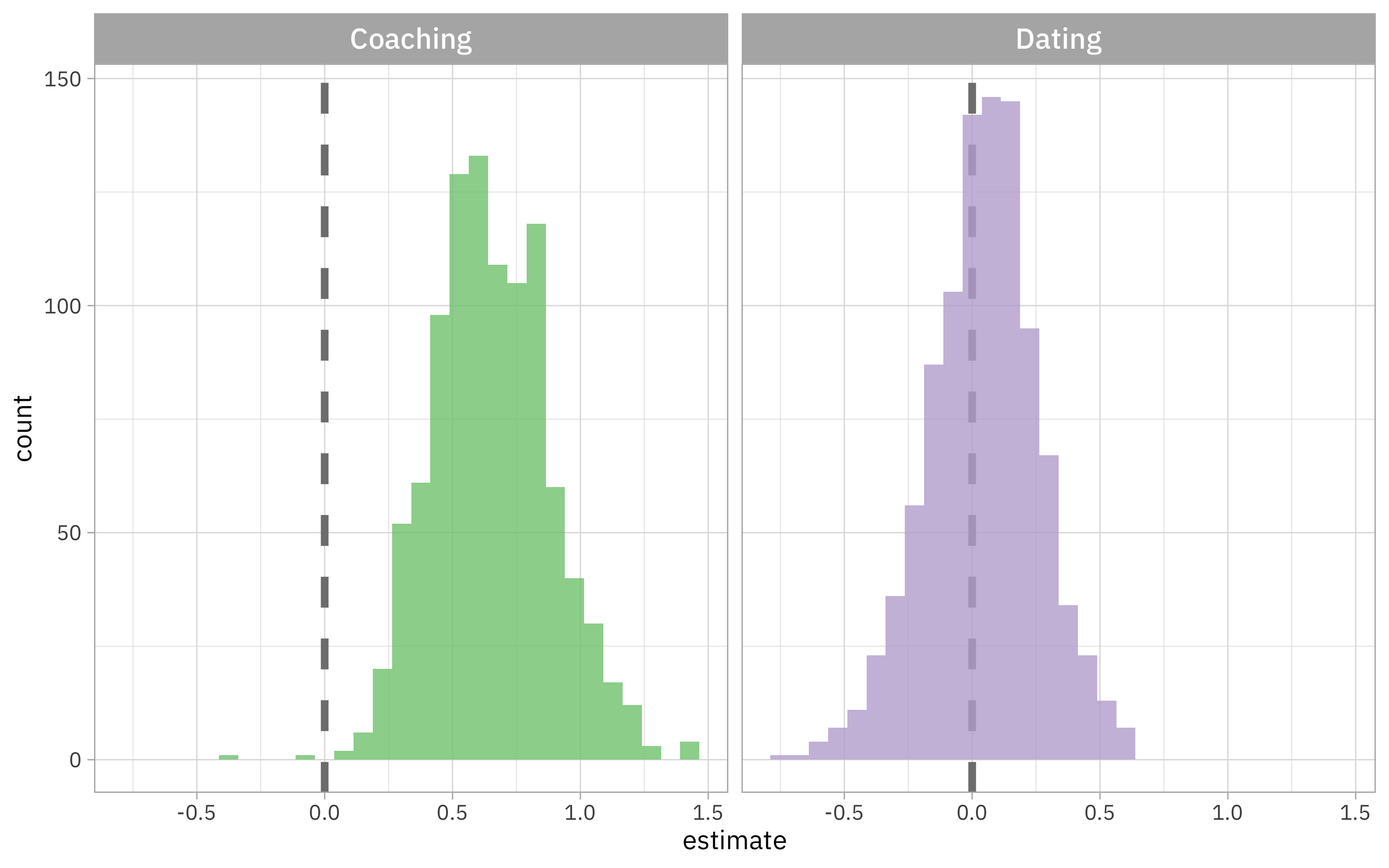
Looks like we have strong evidence that Roy Kent says “F*CK” more per episode when he is coaching, but no real evidence that he does so more or less when dating Keeley.