Sentiment analysis with tidymodels and #TidyTuesday Animal Crossing reviews

A lot has been happening in the tidymodels ecosystem lately! There are many possible projects we on the tidymodels team could focus on next; we are interested in gathering community feedback to inform our priorities. If you are interested in sharing your opinion on next steps in tidymodels development, please take this short survey.

Lately I’ve been publishing screencasts demonstrating how to use the tidymodels framework, from first steps in modeling to how to tune more complex models. Today’s screencast combines one of my favorite topics (text analysis! 📚) with the tidymodels framework, so it is one I am especially happy about.

Here is the code I used in the video, for those who prefer reading instead of or in addition to video.

Explore the data

Our modeling goal is to predict the rating for Animal Crossing user reviews from this week’s #TidyTuesday dataset from the text in the review. This is what is typically called a sentiment analysis model, and it’s a common real-world problem! Let’s get started by looking at the user review data.

library(tidyverse)

user_reviews <- readr::read_tsv("https://raw.githubusercontent.com/rfordatascience/tidytuesday/master/data/2020/2020-05-05/user_reviews.tsv")

user_reviews %>%
  count(grade) %>%
  ggplot(aes(grade, n)) +
  geom_col(fill = "midnightblue", alpha = 0.7)

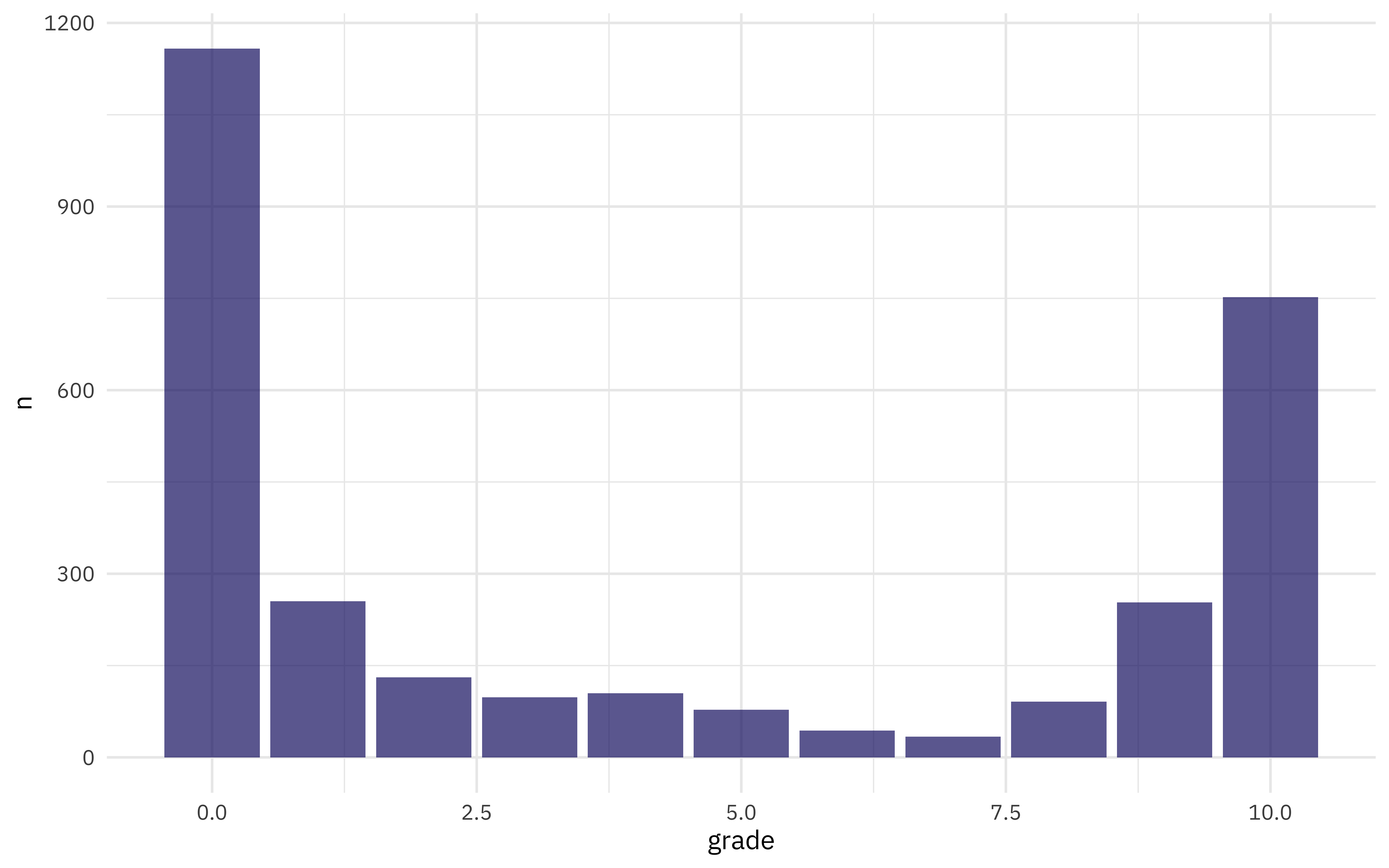
Lots of people give scores of zero, and lots of people give scores of 10. This does not look like a nice distribution for predicting a not-even-really-continuous quantity like this grade, so we’ll convert these user scores to a label, good vs. bad user reviews, and build a classification model.

In the video I used code like the following to look at some example reviews. Actually looking at your data is always a good idea, and this is no less true with text! 📄 A common theme for the negative reviews is frustration with the one-island-per-console setup, and more specifically the relative roles of player 1 vs. others on the same console.

## not run here
user_reviews %>%
  filter(grade > 8) %>%
  sample_n(5) %>%
  pull(text)

We definitely saw some evidence of scraping problems when looking at the review text. Let’s remove at least the final "Expand" from the reviews, and create a new categorical rating variable.

reviews_parsed <- user_reviews %>%
  mutate(text = str_remove(text, "Expand$")) %>%
  mutate(rating = case_when(
    grade > 7 ~ "good",
    TRUE ~ "bad"
  ))

What is the distribution of words per review?

library(tidytext)

words_per_review <- reviews_parsed %>%
  unnest_tokens(word, text) %>%
  count(user_name, name = "total_words")

words_per_review %>%
  ggplot(aes(total_words)) +
  geom_histogram(fill = "midnightblue", alpha = 0.8)

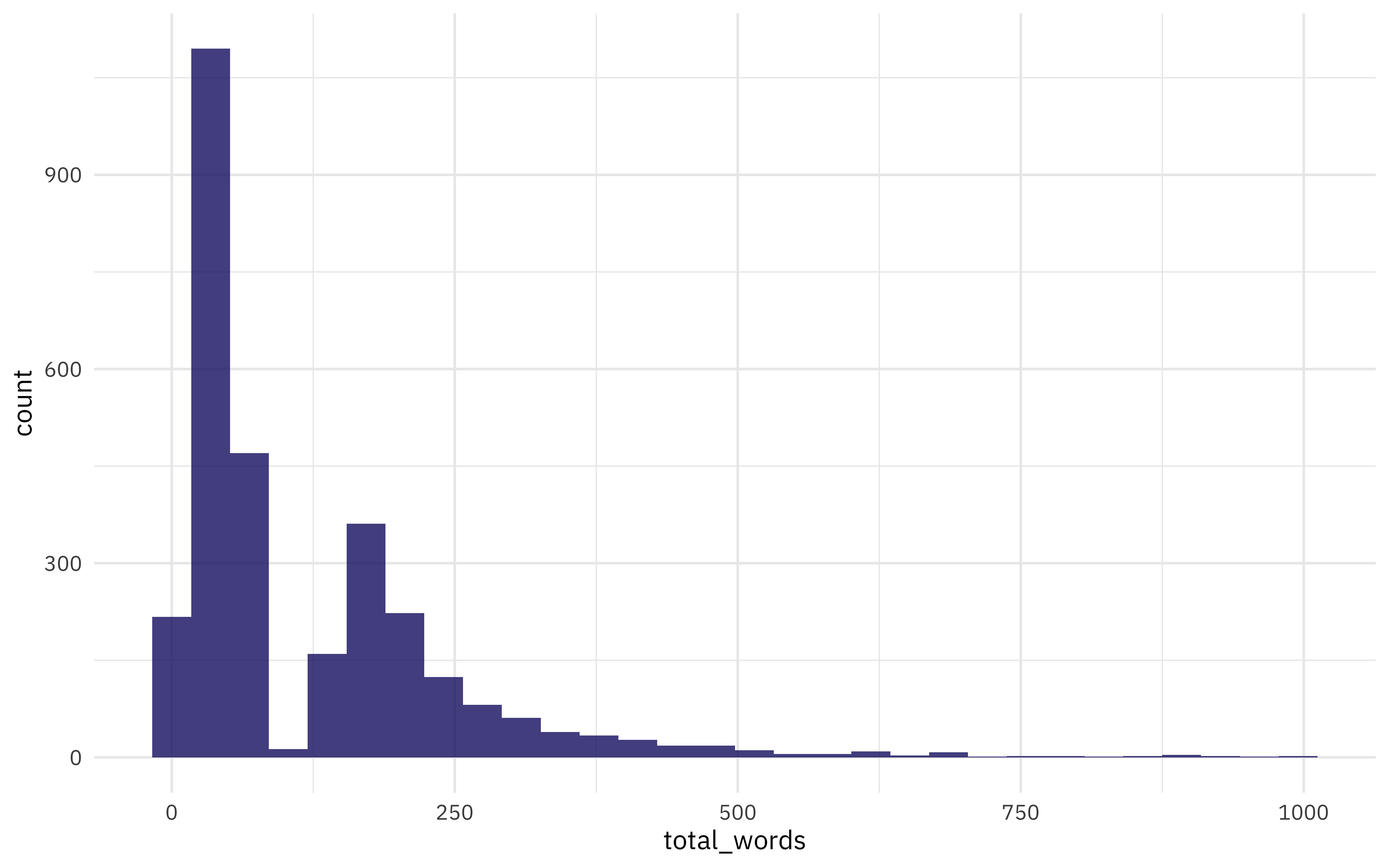
I don’t believe this can be a true, natural distribution of words per review. That sharp drop in the distribution looks very strange and I believe is a sign of some problem with the data generation process (i.e. a scraping problem). That’s life sometimes! Data is never perfect and sometimes we have to do the best we can with the data available. If this was my own project from start-to-finish, I would go back to the scraping and see if I could make any improvements at that stage.

For now, let’s forge ahead and see what we can learn. There are lots more great examples of #TidyTuesday EDA out there to explore, including more text mining!

Build a model

We can start by loading the tidymodels metapackage, and splitting our data into training and testing sets.

library(tidymodels)

set.seed(123)
review_split <- initial_split(reviews_parsed, strata = rating)
review_train <- training(review_split)
review_test <- testing(review_split)

Next, let’s preprocess our data to get it ready for modeling. We can use specialized steps from textrecipes, along with the general recipe steps.

library(textrecipes)

review_rec <- recipe(rating ~ text, data = review_train) %>%
  step_tokenize(text) %>%
  step_stopwords(text) %>%
  step_tokenfilter(text, max_tokens = 500) %>%
  step_tfidf(text) %>%
  step_normalize(all_predictors())

review_prep <- prep(review_rec)

review_prep

## Data Recipe
## 
## Inputs:
## 
##       role #variables
##    outcome          1
##  predictor          1
## 
## Training data contained 2250 data points and no missing data.
## 
## Operations:
## 
## Tokenization for text [trained]
## Stop word removal for text [trained]
## Text filtering for text [trained]
## Term frequency-inverse document frequency with text [trained]
## Centering and scaling for tfidf_text_0, tfidf_text_1, ... [trained]

Let’s walk through the steps in this recipe, which are what I consider sensible defaults for a first attempt at training a text classification model such as a sentiment analysis model.

• First, we must tell the recipe() what our model is going to be (using a formula here) and what data we are using.
• Next, we tokenize our text, with the default tokenization into single words.
• Next, we remove stop words (again, just the default set).
• It wouldn’t be practical to keep all the tokens from this whole dataset in our model, so we can filter down to only keep, in this case, the top 500 most-used tokens (after removing stop words). This is a pretty dramatic cut and keeping more tokens would be a good next step in improving this model.
• We need to decide on some kind of weighting for these tokens next, either something like term frequency or, what we used here, tf-idf.
• Finally, we center and scale (i.e. normalize) all the newly created tf-idf values because the model we are going to use is sensitive to this.

Before using prep() these steps have been defined but not actually run or implemented. The prep() function is where everything gets evaluated.

Now it’s time to specify our model. Here we can set up the model specification for lasso regression with penalty = tune() since we don’t yet know the best value for the regularization parameter and mixture = 1 for lasso. In my experience, the lasso has proved to be a good baseline for text modeling. (And sometimes it is hard to do much better!)

I am using a workflow() in this example for convenience; these are objects that can help you manage modeling pipelines more easily, with pieces that fit together like Lego blocks. This workflow() contains both the recipe and the model.

lasso_spec <- logistic_reg(penalty = tune(), mixture = 1) %>%
  set_engine("glmnet")

lasso_wf <- workflow() %>%
  add_recipe(review_rec) %>%
  add_model(lasso_spec)

lasso_wf

## ══ Workflow ════════════════════════════════════════════════════════════════
## Preprocessor: Recipe
## Model: logistic_reg()
## 
## ── Preprocessor ────────────────────────────────────────────────────────────
## 5 Recipe Steps
## 
## ● step_tokenize()
## ● step_stopwords()
## ● step_tokenfilter()
## ● step_tfidf()
## ● step_normalize()
## 
## ── Model ───────────────────────────────────────────────────────────────────
## Logistic Regression Model Specification (classification)
## 
## Main Arguments:
##   penalty = tune()
##   mixture = 1
## 
## Computational engine: glmnet

Tune model parameters

Let’s get ready to tune the lasso model! First, we need a set of possible regularization parameters to try.

lambda_grid <- grid_regular(penalty(), levels = 40)

Next, we need a set of resampled data to fit and evaluate all these models.

set.seed(123)
review_folds <- bootstraps(review_train, strata = rating)
review_folds

## # Bootstrap sampling using stratification 
## # A tibble: 25 x 2
##    splits             id         
##    <named list>       <chr>      
##  1 <split [2.2K/812]> Bootstrap01
##  2 <split [2.2K/850]> Bootstrap02
##  3 <split [2.2K/814]> Bootstrap03
##  4 <split [2.2K/814]> Bootstrap04
##  5 <split [2.2K/853]> Bootstrap05
##  6 <split [2.2K/840]> Bootstrap06
##  7 <split [2.2K/816]> Bootstrap07
##  8 <split [2.2K/826]> Bootstrap08
##  9 <split [2.2K/804]> Bootstrap09
## 10 <split [2.2K/809]> Bootstrap10
## # … with 15 more rows

Now we can put it all together and implement the tuning. We can set specific metrics to compute during tuning with metric_set(). Let’s look at AUC, positive predictive value, and negative predictive value so we can understand if one class is harder to predict than another.

doParallel::registerDoParallel()

set.seed(2020)
lasso_grid <- tune_grid(
  lasso_wf,
  resamples = review_folds,
  grid = lambda_grid,
  metrics = metric_set(roc_auc, ppv, npv)
)

Once we have our tuning results, we can examine them in detail.

lasso_grid %>%
  collect_metrics()

## # A tibble: 120 x 6
##     penalty .metric .estimator  mean     n std_err
##       <dbl> <chr>   <chr>      <dbl> <int>   <dbl>
##  1 1.00e-10 npv     binary     0.740    25 0.00518
##  2 1.00e-10 ppv     binary     0.864    25 0.00302
##  3 1.00e-10 roc_auc binary     0.878    25 0.00276
##  4 1.80e-10 npv     binary     0.740    25 0.00518
##  5 1.80e-10 ppv     binary     0.864    25 0.00302
##  6 1.80e-10 roc_auc binary     0.878    25 0.00276
##  7 3.26e-10 npv     binary     0.740    25 0.00518
##  8 3.26e-10 ppv     binary     0.864    25 0.00302
##  9 3.26e-10 roc_auc binary     0.878    25 0.00276
## 10 5.88e-10 npv     binary     0.740    25 0.00518
## # … with 110 more rows

Visualization is often more helpful to understand model performance.

lasso_grid %>%
  collect_metrics() %>%
  ggplot(aes(penalty, mean, color = .metric)) +
  geom_line(size = 1.5, show.legend = FALSE) +
  facet_wrap(~.metric) +
  scale_x_log10()

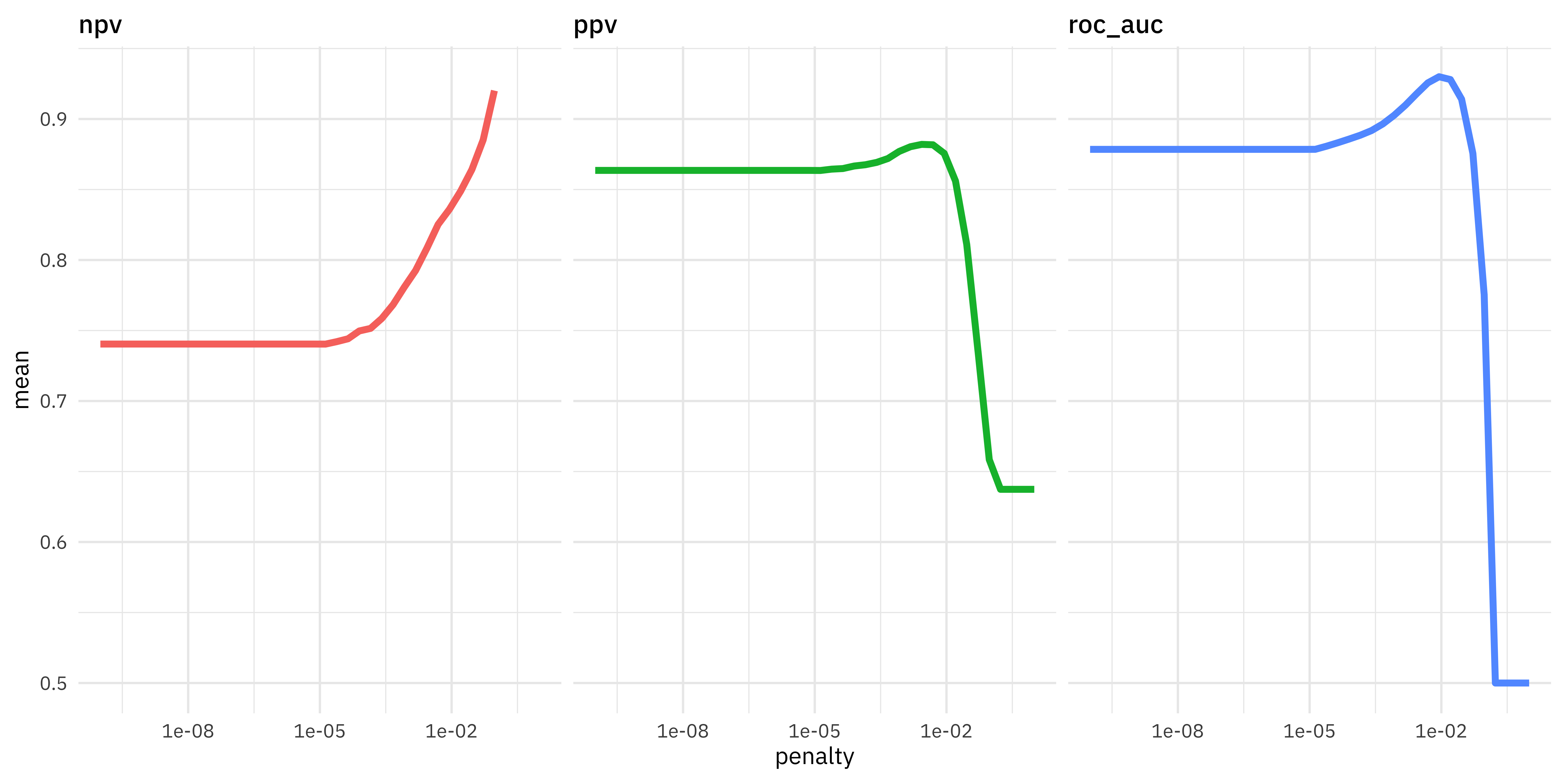
This shows us a lot. We see clearly that AUC and PPV have benefited from the regularization and we could identify the best value of penalty for each of those metrics. The same is not true for NPV. One class (the happy comments) is harder to predict than the other. It might be worth including more tokens in our model, based on this plot.

Choose the final model

Let’s keep our model as is for now, and choose a final model based on AUC. We can use select_best() to find the best AUC and then update our workflow lasso_wf with this value.

best_auc <- lasso_grid %>%
  select_best("roc_auc")

best_auc

## # A tibble: 1 x 1
##   penalty
##     <dbl>
## 1 0.00889

final_lasso <- finalize_workflow(lasso_wf, best_auc)

final_lasso

## ══ Workflow ════════════════════════════════════════════════════════════════
## Preprocessor: Recipe
## Model: logistic_reg()
## 
## ── Preprocessor ────────────────────────────────────────────────────────────
## 5 Recipe Steps
## 
## ● step_tokenize()
## ● step_stopwords()
## ● step_tokenfilter()
## ● step_tfidf()
## ● step_normalize()
## 
## ── Model ───────────────────────────────────────────────────────────────────
## Logistic Regression Model Specification (classification)
## 
## Main Arguments:
##   penalty = 0.00888623816274339
##   mixture = 1
## 
## Computational engine: glmnet

This is our tuned, finalized workflow (but it is not fit yet). One of the things we can do when we start to fit this finalized workflow on the whole training set is to see what the most important variables are using the vip package.

library(vip)

final_lasso %>%
  fit(review_train) %>%
  pull_workflow_fit() %>%
  vi(lambda = best_auc$penalty) %>%
  group_by(Sign) %>%
  top_n(20, wt = abs(Importance)) %>%
  ungroup() %>%
  mutate(
    Importance = abs(Importance),
    Variable = str_remove(Variable, "tfidf_text_"),
    Variable = fct_reorder(Variable, Importance)
  ) %>%
  ggplot(aes(x = Importance, y = Variable, fill = Sign)) +
  geom_col(show.legend = FALSE) +
  facet_wrap(~Sign, scales = "free_y") +
  labs(y = NULL)

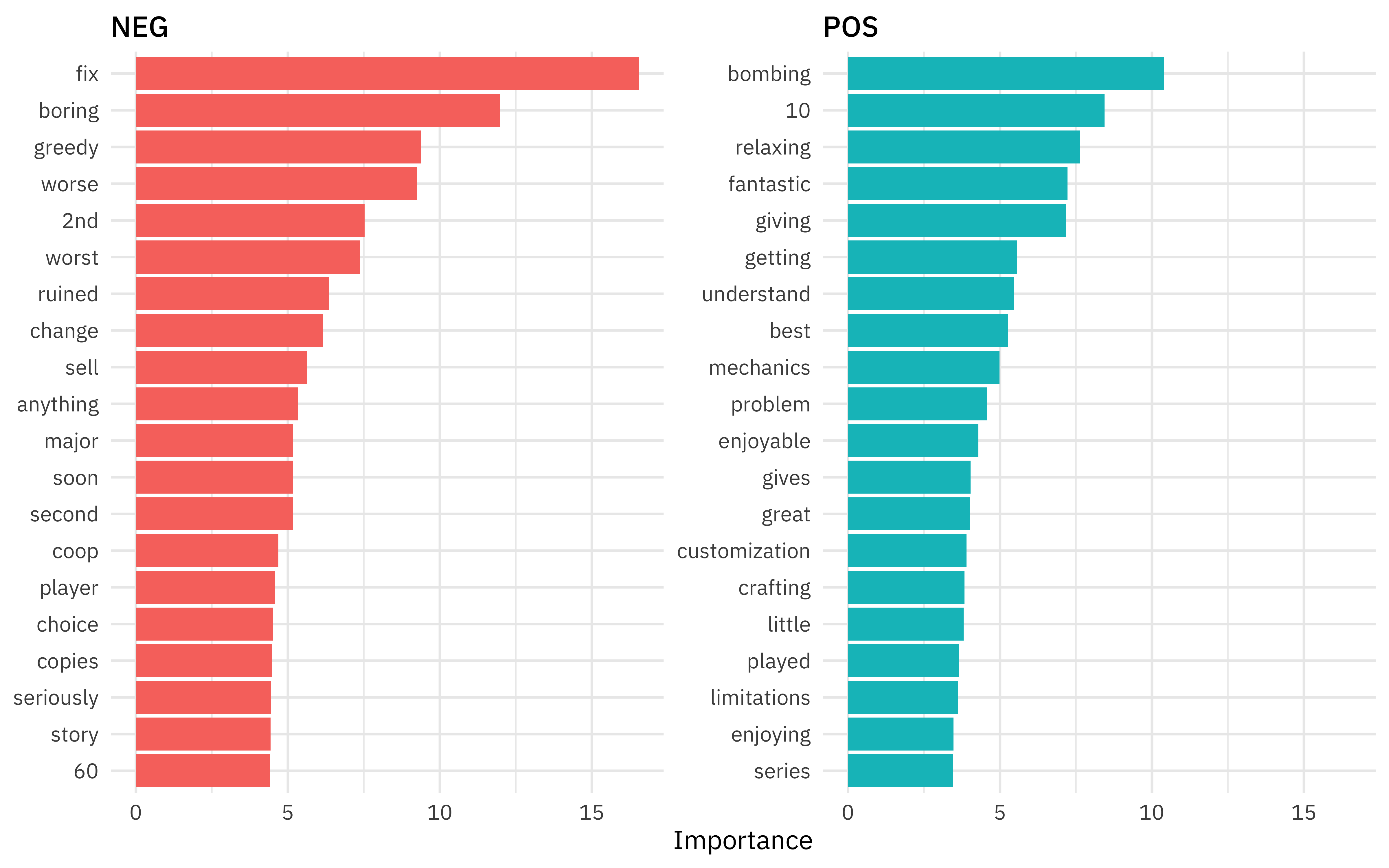
People who are happy with Animal Crossing like to talk about how relaxing, fantastic, enjoyable, and great it is, and also talk in their reviews about the “review bombing” of the negative reviews. Notice that many of the words from the negative reviews are specifically used to talk about the multiplayer experience (it’s boring for the second player, second player cannot do “anything” or move the story forward, cooperative/coop play doesn’t work well, etc). These users want a fix and they declare Nintendo greedy for the one-island-per-console play.

Finally, let’s return to our test data. The tune package has a function last_fit() which is nice for situations when you have tuned and finalized a model or workflow and want to fit it one last time on your training data and evaluate it on your testing data. You only have to pass this function your finalized model/workflow and your split.

review_final <- last_fit(final_lasso, review_split)

review_final %>%
  collect_metrics()

## # A tibble: 2 x 3
##   .metric  .estimator .estimate
##   <chr>    <chr>          <dbl>
## 1 accuracy binary         0.892
## 2 roc_auc  binary         0.941

We did not overfit during our tuning process, and the overall accuracy is not bad. Let’s create a confusion matrix for the testing data.

review_final %>%
  collect_predictions() %>%
  conf_mat(rating, .pred_class)

##           Truth
## Prediction bad good
##       bad  449   55
##       good  26  219

Although our overall accuracy isn’t so bad, we find that it is easier to detect the negative reviews than the positive ones.