Fit and predict with tidymodels for #TidyTuesday bird baths in Australia
By Julia Silge in rstats tidymodels
September 1, 2021
This is the latest in my series of
screencasts demonstrating how to use the
tidymodels packages, from just getting started to tuning more complex models. Today’s screencast is good for folks who are newer to modeling or tidymodels; it focuses on how to use feature engineering together with a model algorithm and how to fit and predict, with this week’s
#TidyTuesday dataset on bird baths in Australia. 🐦
Here is the code I used in the video, for those who prefer reading instead of or in addition to video.
Explore data
Our modeling goal is to predict whether we’ll see a bird at a bird bath in Australia, given info like what kind of bird we’re looking for and whether the bird bath is in an urban or rural location.
library(tidyverse)

bird_baths <- readr::read_csv("https://raw.githubusercontent.com/rfordatascience/tidytuesday/master/data/2021/2021-08-31/bird_baths.csv")

bird_baths %>%
  count(urban_rural)
## # A tibble: 3 × 2
##   urban_rural      n
##   <chr>        <int>
## 1 Rural        49686
## 2 Urban       111202
## 3 <NA>           169
Notice that there are some summary rows in the dataset with NA values for urban_rural, survey_year, etc. We can use that to choose some top bird types to focus on, instead of all the many bird types included in this dataset.
top_birds <-
  bird_baths %>%
  filter(is.na(urban_rural)) %>%
  arrange(-bird_count) %>%
  slice_max(bird_count, n = 15) %>%
  pull(bird_type)

top_birds
##  [1] "Noisy Miner"        "Australian Magpie"  "Rainbow Lorikeet"
##  [4] "Red Wattlebird"     "Superb Fairy-wren"  "Magpie-lark"
##  [7] "Pied Currawong"     "Crimson Rosella"    "Eastern Spinebill"
## [10] "Spotted Dove"       "Lewin's Honeyeater" "Satin Bowerbird"
## [13] "Crested Pigeon"     "Grey Fantail"       "Red-browed Finch"
How likely were the citizen scientists who collected this data to see birds of different types, in different locations?
bird_parsed <-
bird_baths %>%
filter(
!is.na(urban_rural),
bird_type %in% top_birds
) %>%
group_by(urban_rural, bird_type) %>%
summarise(bird_count = mean(bird_count), .groups = "drop")
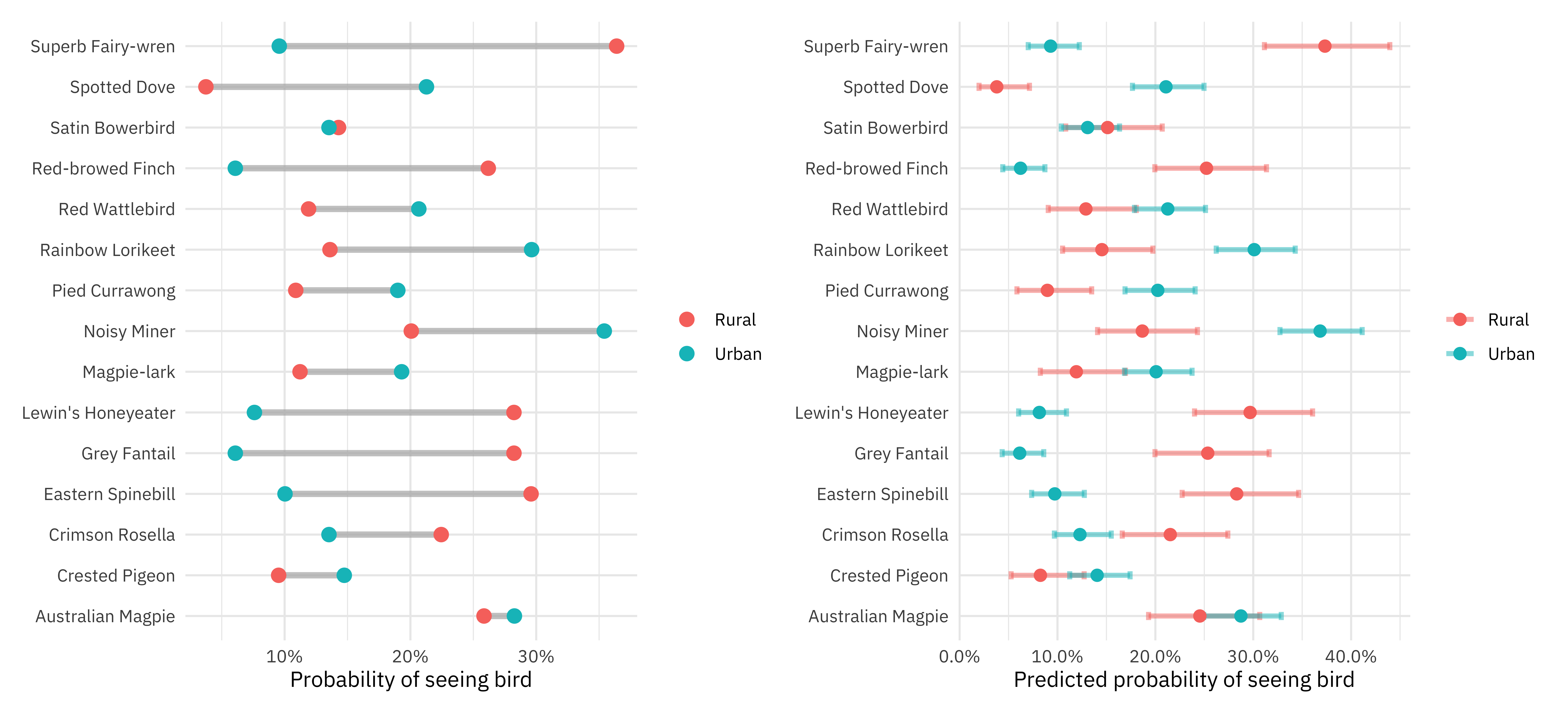
p1 <-
bird_parsed %>%
ggplot(aes(bird_count, bird_type)) +
geom_segment(
data = bird_parsed %>%
pivot_wider(
names_from = urban_rural,
values_from = bird_count
),
aes(x = Rural, xend = Urban, y = bird_type, yend = bird_type),
alpha = 0.7, color = "gray70", size = 1.5
) +
geom_point(aes(color = urban_rural), size = 3) +
scale_x_continuous(labels = scales::percent) +
labs(x = "Probability of seeing bird", y = NULL, color = NULL)
p1
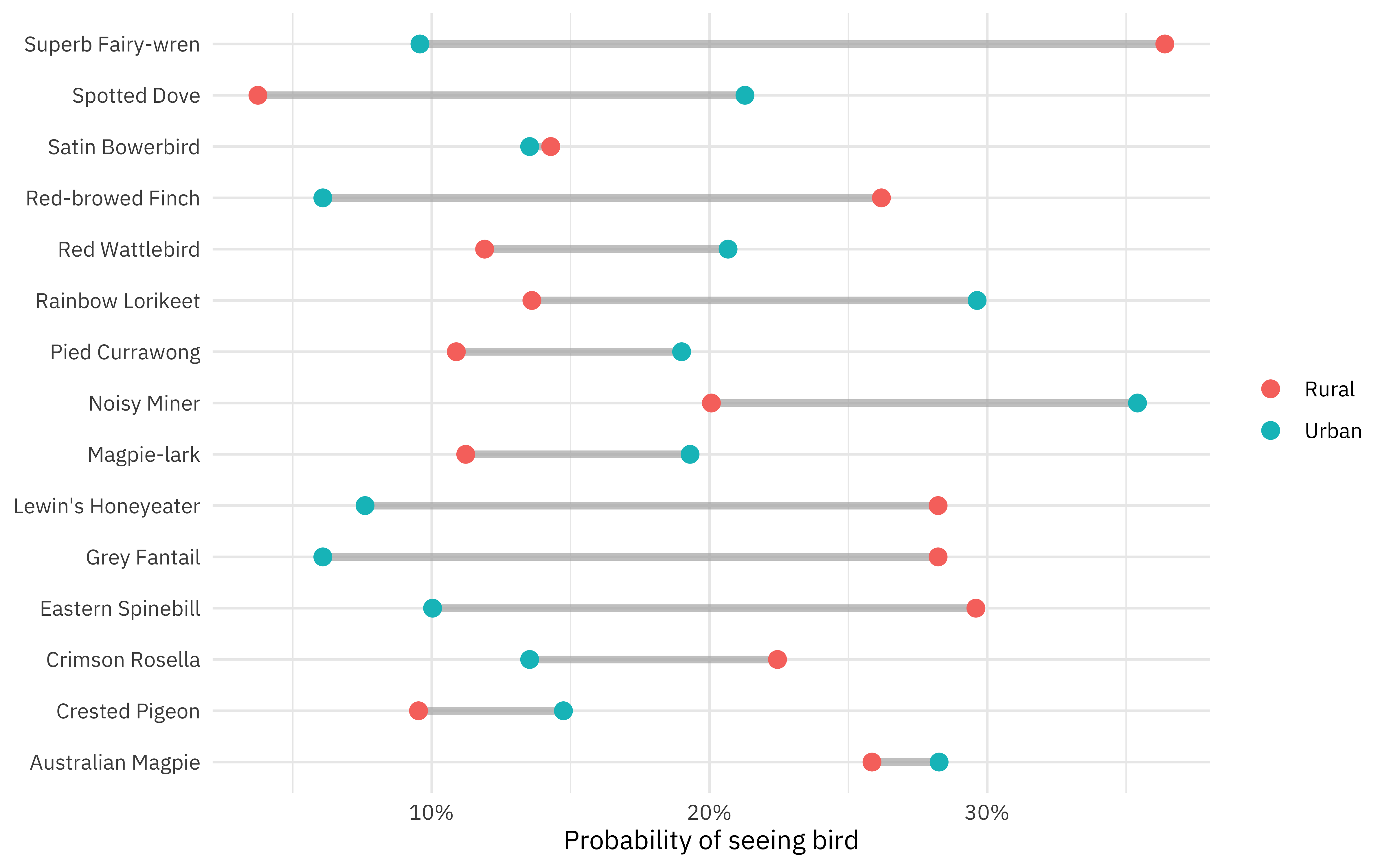
Superb fairy-wrens are more rural, while noisy miners are more urban.
Let’s build a model to predict this probability of seeing a bird using just these two predictors.
bird_df <-
  bird_baths %>%
  filter(
    !is.na(urban_rural),
    bird_type %in% top_birds
  ) %>%
  mutate(bird_count = if_else(bird_count > 0, "bird", "no bird")) %>%
  mutate_if(is.character, as.factor)
Build a first model
Let’s start our modeling by setting up our “data budget.” We are going to use a simple logistic regression model that is unlikely to overfit, but let’s still split our data into training and testing, and then create resampling folds.
library(tidymodels)

set.seed(123)
bird_split <- initial_split(bird_df, strata = bird_count)
bird_train <- training(bird_split)
bird_test <- testing(bird_split)

set.seed(234)
bird_folds <- vfold_cv(bird_train, strata = bird_count)
bird_folds
## #  10-fold cross-validation using stratification
## # A tibble: 10 × 2
##    splits              id
##    <list>              <chr>
##  1 <split [9637/1072]> Fold01
##  2 <split [9638/1071]> Fold02
##  3 <split [9638/1071]> Fold03
##  4 <split [9638/1071]> Fold04
##  5 <split [9638/1071]> Fold05
##  6 <split [9638/1071]> Fold06
##  7 <split [9638/1071]> Fold07
##  8 <split [9638/1071]> Fold08
##  9 <split [9639/1070]> Fold09
## 10 <split [9639/1070]> Fold10
We’ll make a couple of attempts at fitting models here, but they will all use straightforward logistic regression.
glm_spec <- logistic_reg()
For this first model, let’s set up our feature engineering recipe with our outcome and two predictors, and begin with only one preprocessing step to transform our nominal (factor or character, like urban_rural and bird_type) predictors to
dummy or indicator variables. Then let’s put our preprocessing recipe together with our model specification in a workflow.
rec_basic <-
  recipe(bird_count ~ urban_rural + bird_type, data = bird_train) %>%
  step_dummy(all_nominal_predictors())

wf_basic <- workflow(rec_basic, glm_spec)
We could fit this one time to the training data, but to get better estimates of performance, let’s fit 10 times to our 10 resampling folds.
doParallel::registerDoParallel()
ctrl_preds <- control_resamples(save_pred = TRUE)
rs_basic <- fit_resamples(wf_basic, bird_folds, control = ctrl_preds)
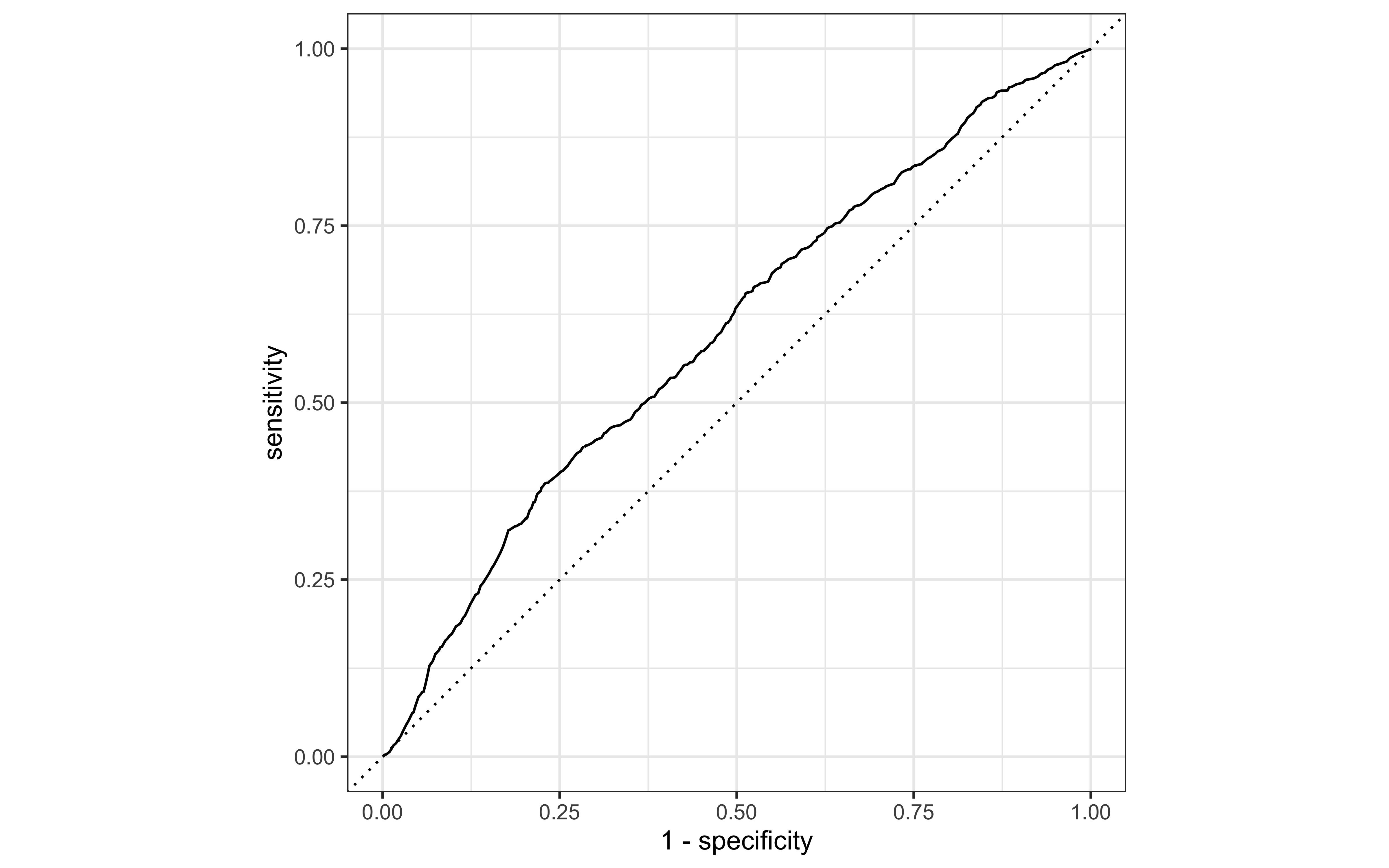
How did this turn out? If we look at some overall metrics, accuracy does not look so bad:
collect_metrics(rs_basic)
## # A tibble: 2 × 6
##   .metric  .estimator  mean     n   std_err .config
##   <chr>    <chr>      <dbl> <int>     <dbl> <chr>
## 1 accuracy binary     0.822    10 0.0000762 Preprocessor1_Model1
## 2 roc_auc  binary     0.601    10 0.00783   Preprocessor1_Model1
This is because there were not many birds overall, though! The model is just saying “no bird” everywhere and getting good accuracy. The ROC curve, on the other hand, looks not so great.
augment(rs_basic) %>%
  roc_curve(bird_count, .pred_bird) %>%
  autoplot()
Add interactions
We know from the plot we made during EDA that there are interactions between whether a bird bath is urban/rural and what kinds of birds we see there; we could model these interactions either with a model type that can handle it natively (like trees) or with explicit interaction terms like this:
rec_interact <-
  rec_basic %>%
  step_interact(~ starts_with("urban_rural"):starts_with("bird_type"))

wf_interact <- workflow(rec_interact, glm_spec)
rs_interact <- fit_resamples(wf_interact, bird_folds, control = ctrl_preds)
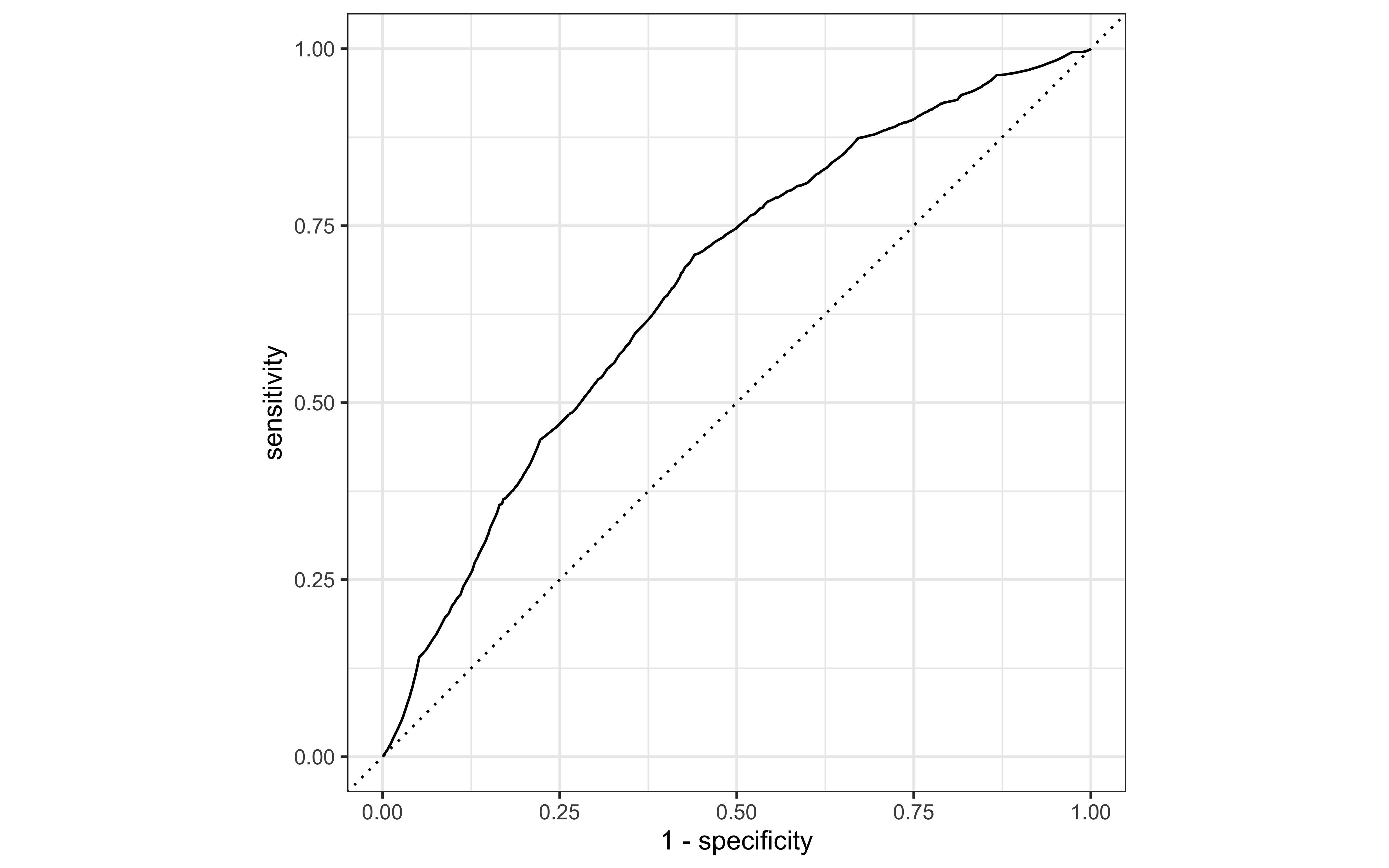
How did this do, our same logistic regression model specification but now with interactions?
collect_metrics(rs_interact)
## # A tibble: 2 × 6
##   .metric  .estimator  mean     n   std_err .config
##   <chr>    <chr>      <dbl> <int>     <dbl> <chr>
## 1 accuracy binary     0.822    10 0.0000762 Preprocessor1_Model1
## 2 roc_auc  binary     0.669    10 0.00660   Preprocessor1_Model1
The accuracy is about the same (since the model is always predicting “no bird”) but the probabilities look better.
augment(rs_interact) %>%
  roc_curve(bird_count, .pred_bird) %>%
  autoplot()
Evaluate model on new data
Let’s stick with this model, logistic regression together with interactions between urban/rural and bird type. We can fit the model one time to the entire training set.
bird_fit <- fit(wf_interact, bird_train)
Now this trained model is ready to be applied to new data. For example, we can predict the test set, perhaps to get out probabilities.
predict(bird_fit, bird_test, type = "prob")
## # A tibble: 3,571 × 2
##    .pred_bird `.pred_no bird`
##         <dbl>           <dbl>
##  1     0.213            0.787
##  2     0.123            0.877
##  3     0.141            0.859
##  4     0.283            0.717
##  5     0.119            0.881
##  6     0.252            0.748
##  7     0.0380           0.962
##  8     0.123            0.877
##  9     0.129            0.871
## 10     0.119            0.881
## # … with 3,561 more rows
In fact, we can predict on any kind of new data that has the right input variables. Let’s make some ourselves.
new_bird_data <-
  tibble(bird_type = top_birds) %>%
  crossing(urban_rural = c("Urban", "Rural"))

new_bird_data
## # A tibble: 30 × 2
##    bird_type         urban_rural
##    <chr>             <chr>
##  1 Australian Magpie Rural
##  2 Australian Magpie Urban
##  3 Crested Pigeon    Rural
##  4 Crested Pigeon    Urban
##  5 Crimson Rosella   Rural
##  6 Crimson Rosella   Urban
##  7 Eastern Spinebill Rural
##  8 Eastern Spinebill Urban
##  9 Grey Fantail      Rural
## 10 Grey Fantail      Urban
## # … with 20 more rows
We can use a
helpful function like augment() to take this new data and “augment” it with predicted probabilities and class predictions, and we can
use predict() with specific type arguments to return specialized predictions like confidence intervals. Let’s bind these together.
bird_preds <-
  augment(bird_fit, new_bird_data) %>%
  bind_cols(
    predict(bird_fit, new_bird_data, type = "conf_int")
  )

bird_preds
## # A tibble: 30 × 9
##    bird_type urban_rural .pred_class .pred_bird `.pred_no bird` .pred_lower_bird
##    <chr>     <chr>       <fct>            <dbl>           <dbl>            <dbl>
##  1 Australi… Rural       no bird         0.245            0.755           0.193
##  2 Australi… Urban       no bird         0.287            0.713           0.249
##  3 Crested … Rural       no bird         0.0826           0.917           0.0526
##  4 Crested … Urban       no bird         0.141            0.859           0.113
##  5 Crimson … Rural       no bird         0.215            0.785           0.166
##  6 Crimson … Urban       no bird         0.123            0.877           0.0969
##  7 Eastern … Rural       no bird         0.283            0.717           0.227
##  8 Eastern … Urban       no bird         0.0973           0.903           0.0736
##  9 Grey Fan… Rural       no bird         0.254            0.746           0.200
## 10 Grey Fan… Urban       no bird         0.0614           0.939           0.0435
## # … with 20 more rows, and 3 more variables: .pred_upper_bird <dbl>,
## #   .pred_lower_no bird <dbl>, .pred_upper_no bird <dbl>
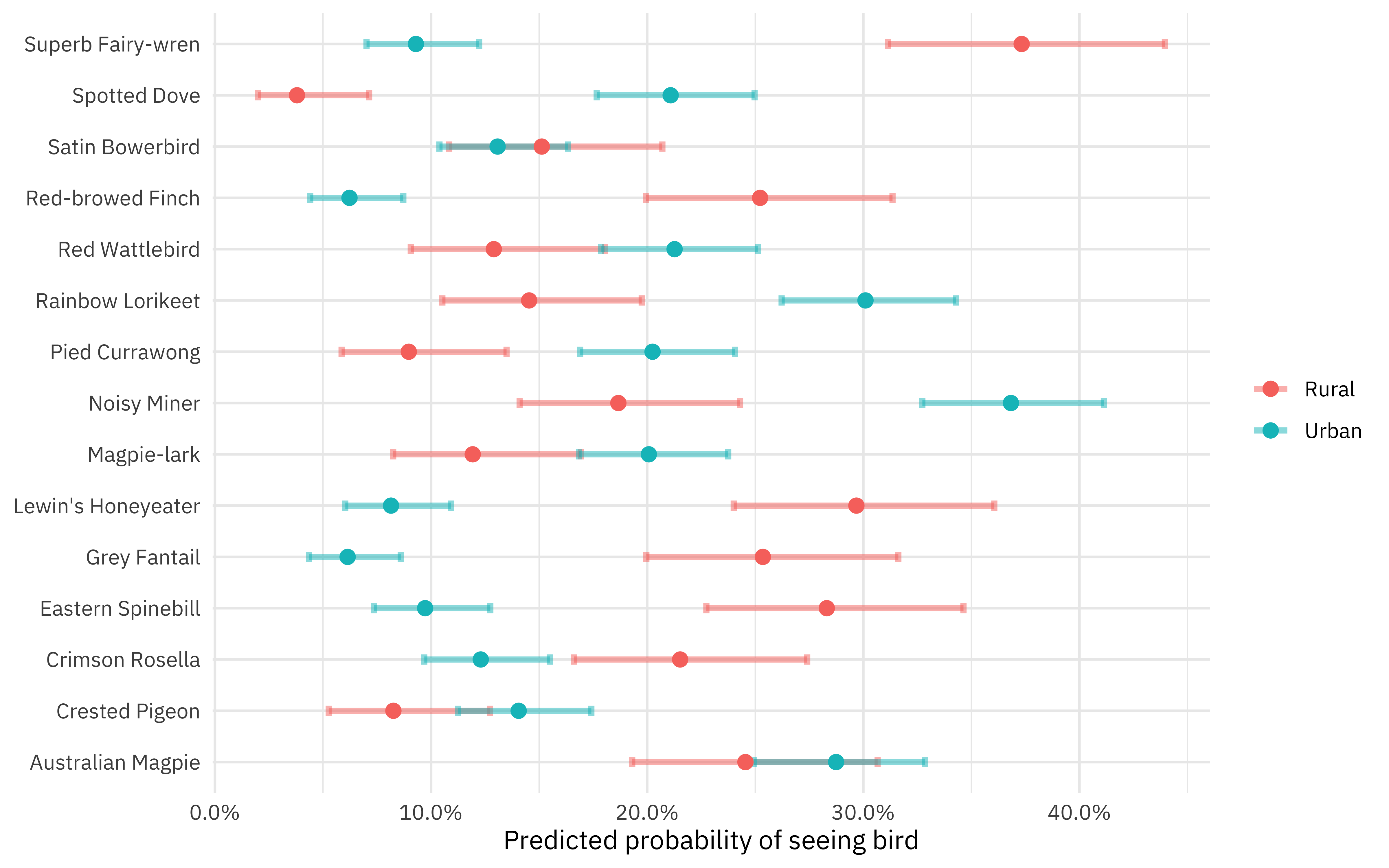
Now let’s visualize these predictions.
p2 <-
  bird_preds %>%
  ggplot(aes(.pred_bird, bird_type, color = urban_rural)) +
  geom_errorbar(aes(
    xmin = .pred_lower_bird,
    xmax = .pred_upper_bird
  ),
  width = .2, size = 1.2, alpha = 0.5
  ) +
  geom_point(size = 2.5) +
  scale_x_continuous(labels = scales::percent) +
  labs(x = "Predicted probability of seeing bird", y = NULL, color = NULL)

p2
Actually, let’s put this together with our earlier plot!
library(patchwork)

p1 + p2
- Posted on:
- September 1, 2021
- Length:
- 7 minute read, 1416 words
- Categories:
- rstats tidymodels
- Tags:
- rstats tidymodels