Logistic regression modeling for #TidyTuesday US House Elections
By Julia Silge in rstats
November 7, 2023
This is the latest in my series of
screencasts! Today is Election Day in the United States, and this screencast focuses on logistic regression modeling with this week’s
#TidyTuesday dataset on US House Election Results. 🇺🇸
Here is the code I used in the video, for those who prefer reading instead of or in addition to video. FYI, I recently started using GitHub Copilot in RStudio and you can see it in action in the video.
Explore data
This screencast doesn’t use tidymodels, but just plain old glm(). In this case, I don’t have any preprocessing or resampling needs and the
particular way I want to use glm() isn’t supported yet in tidymodels. Our modeling goal is to understand vote share in the
US House election results. Let’s start by reading in the data:
library(tidyverse)
house <- read_csv('https://raw.githubusercontent.com/rfordatascience/tidytuesday/master/data/2023/2023-11-07/house.csv')
glimpse(house)
## Rows: 32,452
## Columns: 20
## $ year           <dbl> 1976, 1976, 1976, 1976, 1976, 1976, 1976, 1976, 1976, 1…
## $ state          <chr> "ALABAMA", "ALABAMA", "ALABAMA", "ALABAMA", "ALABAMA", …
## $ state_po       <chr> "AL", "AL", "AL", "AL", "AL", "AL", "AL", "AL", "AL", "…
## $ state_fips     <dbl> 1, 1, 1, 1, 1, 1, 1, 1, 1, 1, 1, 1, 1, 1, 1, 1, 1, 1, 1…
## $ state_cen      <dbl> 63, 63, 63, 63, 63, 63, 63, 63, 63, 63, 63, 63, 63, 63,…
## $ state_ic       <dbl> 41, 41, 41, 41, 41, 41, 41, 41, 41, 41, 41, 41, 41, 41,…
## $ office         <chr> "US HOUSE", "US HOUSE", "US HOUSE", "US HOUSE", "US HOU…
## $ district       <chr> "001", "001", "001", "002", "002", "002", "003", "003",…
## $ stage          <chr> "GEN", "GEN", "GEN", "GEN", "GEN", "GEN", "GEN", "GEN",…
## $ runoff         <lgl> FALSE, FALSE, FALSE, FALSE, FALSE, FALSE, FALSE, FALSE,…
## $ special        <lgl> FALSE, FALSE, FALSE, FALSE, FALSE, FALSE, FALSE, FALSE,…
## $ candidate      <chr> "BILL DAVENPORT", "JACK EDWARDS", "WRITEIN", "J CAROLE …
## $ party          <chr> "DEMOCRAT", "REPUBLICAN", NA, "DEMOCRAT", "REPUBLICAN",…
## $ writein        <lgl> FALSE, FALSE, TRUE, FALSE, FALSE, TRUE, FALSE, FALSE, T…
## $ mode           <chr> "TOTAL", "TOTAL", "TOTAL", "TOTAL", "TOTAL", "TOTAL", "…
## $ candidatevotes <dbl> 58906, 98257, 7, 66288, 90069, 5, 106935, 1111, 2, 3453…
## $ totalvotes     <dbl> 157170, 157170, 157170, 156362, 156362, 156362, 108048,…
## $ unofficial     <lgl> FALSE, FALSE, FALSE, FALSE, FALSE, FALSE, FALSE, FALSE,…
## $ version        <dbl> 20230706, 20230706, 20230706, 20230706, 20230706, 20230…
## $ fusion_ticket  <lgl> FALSE, FALSE, FALSE, FALSE, FALSE, FALSE, FALSE, FALSE,…
How many different political parties are represented in these elections?
house |>
    count(party, sort = TRUE)
## # A tibble: 478 × 2
##    party                n
##    <chr>            <int>
##  1 DEMOCRAT          9908
##  2 REPUBLICAN        9705
##  3 <NA>              3858
##  4 LIBERTARIAN       2769
##  5 INDEPENDENT       1217
##  6 CONSERVATIVE       668
##  7 GREEN              513
##  8 NATURAL LAW        371
##  9 WORKING FAMILIES   283
## 10 LIBERAL            266
## # ℹ 468 more rows
A ton, but we probably want to focus on the two main political parties in the US. How does vote share in a given election look for the two parties?
house |>
    filter(party %in% c("DEMOCRAT", "REPUBLICAN")) |>
    ggplot(aes(candidatevotes / totalvotes, fill = party)) +
    geom_histogram(position = "identity", bins = 40, alpha = 0.7) +
    scale_x_continuous(labels = scales::percent_format()) +
    labs(x = "% of total votes", y = "Number of elections", fill = NULL)
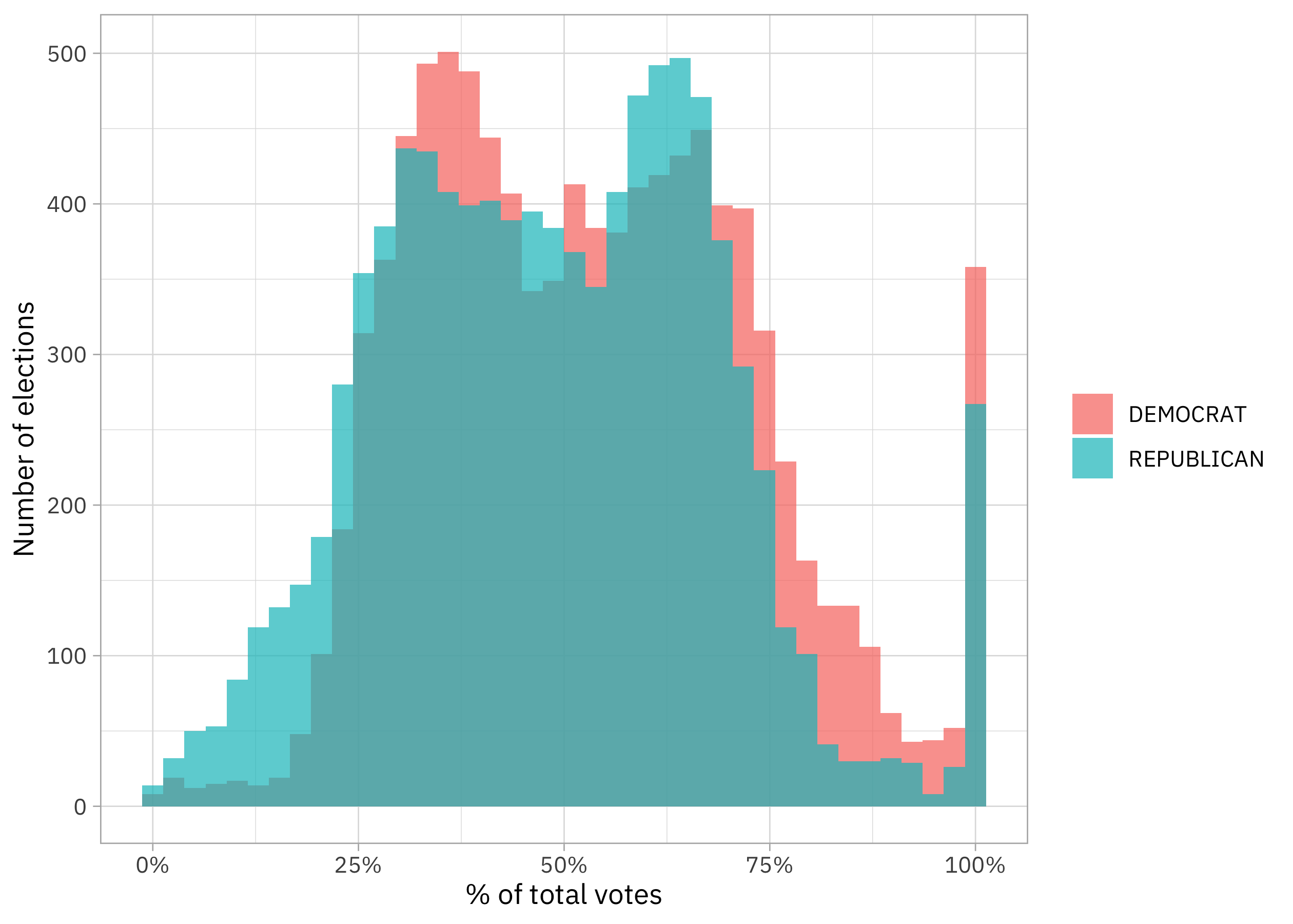
For the time period as a whole, vote share for Democrats is shifted to higher values than for Republicans at the tails (less close elections) while the opposite is true nearer the middle (more close elections). That’s quite an interesting distribution, if you ask me.
Has vote share changed over time?
house |>
    filter(party %in% c("DEMOCRAT", "REPUBLICAN")) |>
    ggplot(aes(year, candidatevotes / totalvotes, fill = factor(year))) +
    geom_boxplot(alpha = 0.8, show.legend = FALSE) +
    scale_y_continuous(labels = scales::percent_format()) +
    scale_fill_viridis_d() +
    labs(x = NULL, y = "% of total votes", fill = NULL)
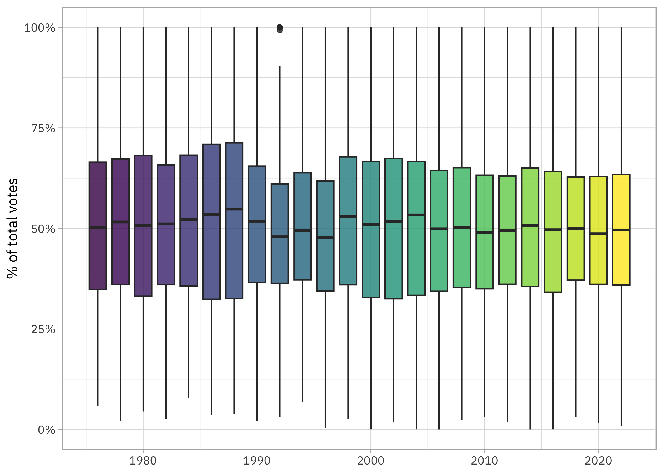
It looks to me like vote share may be decreasing overall over time, indicating closer elections. However, I’d like to use modeling to understand this better. I’m especially interested in whether the relationship is different for Democrats and Republicans.
Logistic regression model
Let’s only use the election results for Democrat and Republication candidates in our model:
house_subset <-
    house |>
    filter(party %in% c("DEMOCRAT", "REPUBLICAN"))
Remember that we have candidatevotes and totalvotes for each candidate. You’re probably familiar with using glm() for logistic regression for a binary outcome (like “won” and “lost”) but you can also use it with cbind() syntax for the outcome to model a matrix of successes and failures. I have found this really useful in many real world situations where you are dealing with a proportion, as with this vote share data. You can look at the docs for glm() to learn more, but what we want is a two-column matrix with columns for the numbers of “successes” (candidate votes in this example) and “failures” (votes for people other than this candidate).
house_mod <-
    glm(cbind(candidatevotes, totalvotes - candidatevotes + 1) ~
            party + year + state_po,
        data = house_subset, family = binomial())
I added the + 1 here as an easy way to handle the elections where a candidate won all votes. This model can’t handle zeroes for “failures” but I don’t want to drop those elections from the model.
summary(house_mod)
##
## Call:
## glm(formula = cbind(candidatevotes, totalvotes - candidatevotes +
##     1) ~ party + year + state_po, family = binomial(), data = house_subset)
##
## Coefficients:
##                   Estimate Std. Error  z value Pr(>|z|)
## (Intercept)      2.988e+00  4.569e-03   653.82   <2e-16 ***
## partyREPUBLICAN -7.959e-02  6.236e-05 -1276.26   <2e-16 ***
## year            -1.542e-03  2.263e-06  -681.37   <2e-16 ***
## state_poAL       4.209e-01  6.497e-04   647.90   <2e-16 ***
## state_poAR       2.365e-01  6.893e-04   343.14   <2e-16 ***
## state_poAZ       1.503e-01  6.381e-04   235.49   <2e-16 ***
## state_poCA       1.275e-01  5.978e-04   213.23   <2e-16 ***
## state_poCO       1.019e-01  6.322e-04   161.12   <2e-16 ***
## state_poCT       6.004e-02  6.439e-04    93.24   <2e-16 ***
## state_poDC      -7.689e-01  2.248e-03  -341.99   <2e-16 ***
## state_poDE       1.047e-01  8.086e-04   129.44   <2e-16 ***
## state_poFL       2.079e-01  6.064e-04   342.91   <2e-16 ***
## state_poGA       3.148e-01  6.232e-04   505.12   <2e-16 ***
## state_poHI       1.014e-01  7.648e-04   132.64   <2e-16 ***
## state_poIA       1.295e-01  6.476e-04   199.96   <2e-16 ***
## state_poID       9.791e-02  7.241e-04   135.21   <2e-16 ***
## state_poIL       1.669e-01  6.076e-04   274.74   <2e-16 ***
## state_poIN       1.087e-01  6.247e-04   174.07   <2e-16 ***
## state_poKS       1.634e-01  6.632e-04   246.44   <2e-16 ***
## state_poKY       2.042e-01  6.468e-04   315.68   <2e-16 ***
## state_poLA      -6.333e-01  6.500e-04  -974.33   <2e-16 ***
## state_poMA       3.427e-01  6.252e-04   548.15   <2e-16 ***
## state_poMD       1.046e-01  6.290e-04   166.35   <2e-16 ***
## state_poME       5.382e-02  6.869e-04    78.36   <2e-16 ***
## state_poMI       1.209e-01  6.097e-04   198.25   <2e-16 ***
## state_poMN       7.655e-02  6.363e-04   120.31   <2e-16 ***
## state_poMO       1.054e-01  6.238e-04   168.99   <2e-16 ***
## state_poMS       2.073e-01  6.769e-04   306.30   <2e-16 ***
## state_poMT       7.755e-02  7.482e-04   103.66   <2e-16 ***
## state_poNC       1.688e-01  6.169e-04   273.55   <2e-16 ***
## state_poND       1.639e-01  8.302e-04   197.37   <2e-16 ***
## state_poNE       1.696e-01  6.950e-04   244.00   <2e-16 ***
## state_poNH       9.174e-02  7.260e-04   126.37   <2e-16 ***
## state_poNJ       1.133e-01  6.168e-04   183.65   <2e-16 ***
## state_poNM       1.415e-01  7.076e-04   199.96   <2e-16 ***
## state_poNV       6.186e-02  7.040e-04    87.86   <2e-16 ***
## state_poNY      -1.406e-01  6.031e-04  -233.18   <2e-16 ***
## state_poOH       1.440e-01  6.077e-04   236.96   <2e-16 ***
## state_poOK       1.355e-01  6.573e-04   206.09   <2e-16 ***
## state_poOR       1.225e-01  6.406e-04   191.17   <2e-16 ***
## state_poPA       2.200e-01  6.072e-04   362.31   <2e-16 ***
## state_poRI       1.004e-01  7.608e-04   131.96   <2e-16 ***
## state_poSC       2.450e-01  6.503e-04   376.81   <2e-16 ***
## state_poSD       1.695e-01  7.887e-04   214.93   <2e-16 ***
## state_poTN       2.259e-01  6.353e-04   355.53   <2e-16 ***
## state_poTX       2.379e-01  6.044e-04   393.52   <2e-16 ***
## state_poUT       7.721e-02  6.833e-04   113.00   <2e-16 ***
## state_poVA       2.731e-01  6.240e-04   437.61   <2e-16 ***
## state_poVT      -2.115e-01  8.717e-04  -242.62   <2e-16 ***
## state_poWA       1.358e-01  6.225e-04   218.22   <2e-16 ***
## state_poWI       2.036e-01  6.238e-04   326.40   <2e-16 ***
## state_poWV       2.498e-01  7.163e-04   348.75   <2e-16 ***
## state_poWY       3.970e-02  8.805e-04    45.09   <2e-16 ***
## ---
## Signif. codes:  0 '***' 0.001 '**' 0.01 '*' 0.05 '.' 0.1 ' ' 1
##
## (Dispersion parameter for binomial family taken to be 1)
##
##     Null deviance: 644839486  on 19611  degrees of freedom
## Residual deviance: 622385502  on 19559  degrees of freedom
## AIC: 622624777
##
## Number of Fisher Scoring iterations: 4
We can use tidy() from the broom package to get the model coefficients into a tidy data frame.
library(broom)
tidy(house_mod)
## # A tibble: 53 × 5
##    term            estimate  std.error statistic p.value
##    <chr>              <dbl>      <dbl>     <dbl>   <dbl>
##  1 (Intercept)      2.99    0.00457        654.        0
##  2 partyREPUBLICAN -0.0796  0.0000624    -1276.        0
##  3 year            -0.00154 0.00000226    -681.        0
##  4 state_poAL       0.421   0.000650       648.        0
##  5 state_poAR       0.237   0.000689       343.        0
##  6 state_poAZ       0.150   0.000638       235.        0
##  7 state_poCA       0.127   0.000598       213.        0
##  8 state_poCO       0.102   0.000632       161.        0
##  9 state_poCT       0.0600  0.000644        93.2       0
## 10 state_poDC      -0.769   0.00225       -342.        0
## # ℹ 43 more rows
That’s great and all, but I’ll be honest that those model coefficients on the logistic scale aren’t always super easy to interpret for me. What I often will do is make up some new data spanning the variables of interest, use augment() from the broom package to get the predictions from the model for this new data, and then make a visualization.
new_data <-
    crossing(party = c("DEMOCRAT", "REPUBLICAN"),
             state_po = unique(house_subset$state_po),
             year = 1975:2022)

augment(house_mod, newdata = new_data, type.predict = "response") |>
    mutate(group = paste(party, state_po, sep = "_")) |>
    ggplot(aes(year, .fitted, group = group, color = party)) +
    geom_hline(yintercept = 0.5, linetype = "dashed", alpha = 0.5, size = 2, color = "gray50") +
    geom_line(alpha = 0.4, size = 1.4, show.legend = FALSE) +
    scale_y_continuous(labels = scales::percent_format()) +
    facet_wrap(vars(party)) +
    labs(x = NULL, y = "% of total votes", color = NULL)
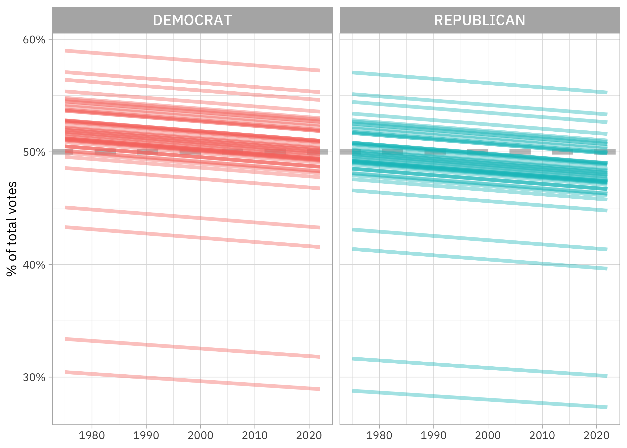
This was a linear model on the logistic scale, and notice how clearly we see that here. The slopes are the same for Democrats and Republicans, but the intercepts are different. Democrats have a higher vote share overall, but the vote share for both parties is going down over time.
What about interactions?
The assumptions we made when set up the predictors like party + year + state_po are probably not very good. I think it’s unlikely the relationship between year and vote share are the same for Democrats and Republicans. We can add an interaction term to the model to allow for this, and then make the same plot using augment(). I find this approach of augment() plus visualization to be especially helpful with interactions and other more complex models. I don’t know about you, but I can’t look at a table of model coefficients with interaction terms and understand what they mean directly. A visualization can be quite clear, by contrast:
house_interact <-
    glm(cbind(candidatevotes, totalvotes - candidatevotes + 1) ~
            party * year + state_po,
        data = house_subset, family = binomial())

augment(house_interact, newdata = new_data, type.predict = "response") |>
    mutate(group = paste(party, state_po, sep = "_")) |>
    ggplot(aes(year, .fitted, group = group, color = party)) +
    geom_hline(yintercept = 0.5, linetype = "dashed", alpha = 0.5, size = 2, color = "gray50") +
    geom_line(alpha = 0.4, size = 1.4, show.legend = FALSE) +
    scale_y_continuous(labels = scales::percent_format()) +
    facet_wrap(vars(party)) +
    labs(x = NULL, y = "% of total votes", color = NULL)
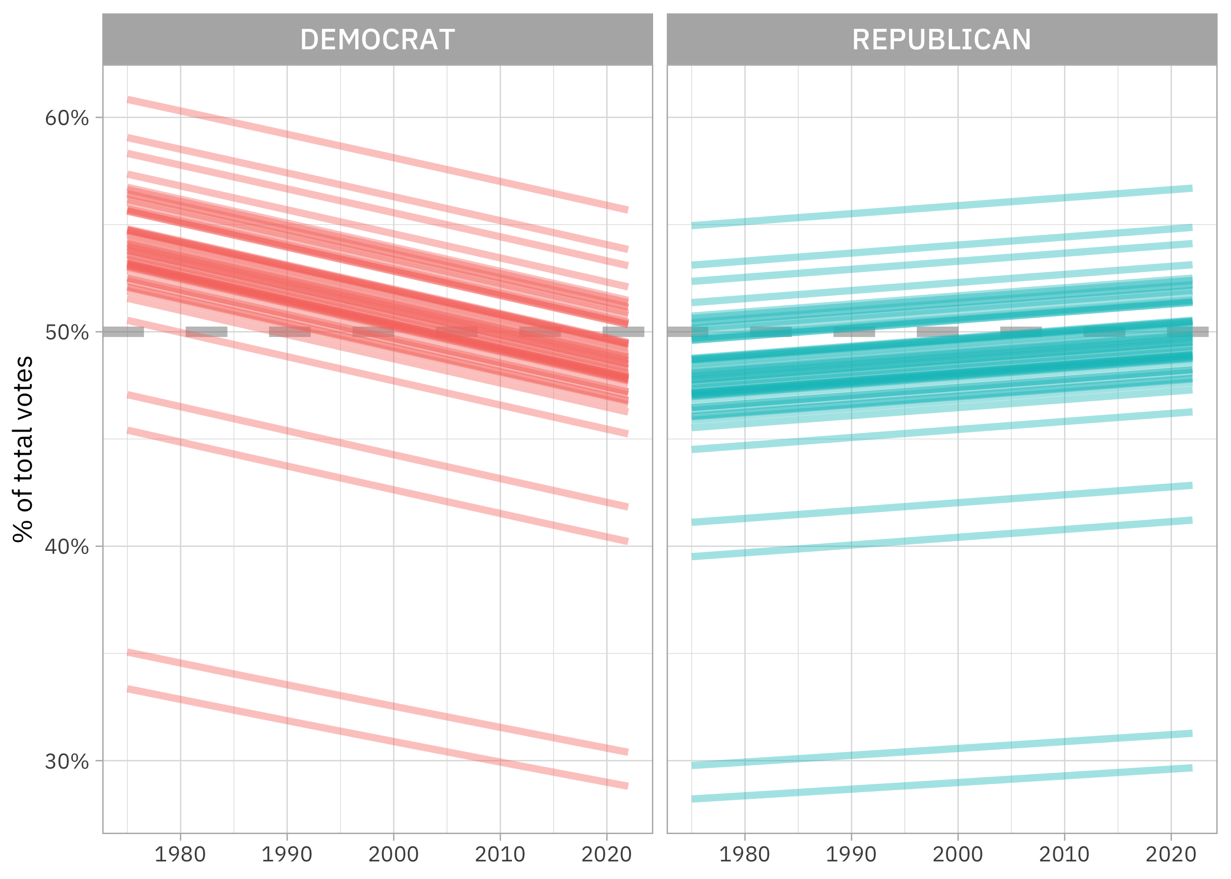
Notice that the slopes are now different for Democrats and Republicans; that’s what the interaction in the model does. The vote share for Democrats in US House Elections is decreasing over time, while the vote share for Republicans is increasing (although not as fast). There are a lot of complex circumstances that go into the “real” reasons for why we see this change, including how the boundaries of US House Districts have changed over this time period. We could try a three-way interaction with party * year * state_po but in my experience, three-way interactions are often not very practically useful. Take a look at the video if you want to see the spaghetti plot that results from that model! 😆