Tune random forests for #TidyTuesday IKEA prices

This is the latest in my series of screencasts demonstrating how to use the tidymodels packages, from starting out with first modeling steps to tuning more complex models. Today’s screencast walks through how to get started quickly with tidymodels via usemodels functions for code scaffolding and generation, using this week’s #TidyTuesday dataset on IKEA furniture prices. 🛋

Here is the code I used in the video, for those who prefer reading instead of or in addition to video.

Explore the data

Our modeling goal is to predict the price of IKEA furniture from other furniture characteristics like category and size. Let’s start by reading in the data.

library(tidyverse)
ikea <- read_csv("https://raw.githubusercontent.com/rfordatascience/tidytuesday/master/data/2020/2020-11-03/ikea.csv")

How is the price related to the furniture dimensions?

ikea %>%
  select(X1, price, depth:width) %>%
  pivot_longer(depth:width, names_to = "dim") %>%
  ggplot(aes(value, price, color = dim)) +
  geom_point(alpha = 0.4, show.legend = FALSE) +
  scale_y_log10() +
  facet_wrap(~dim, scales = "free_x") +
  labs(x = NULL)

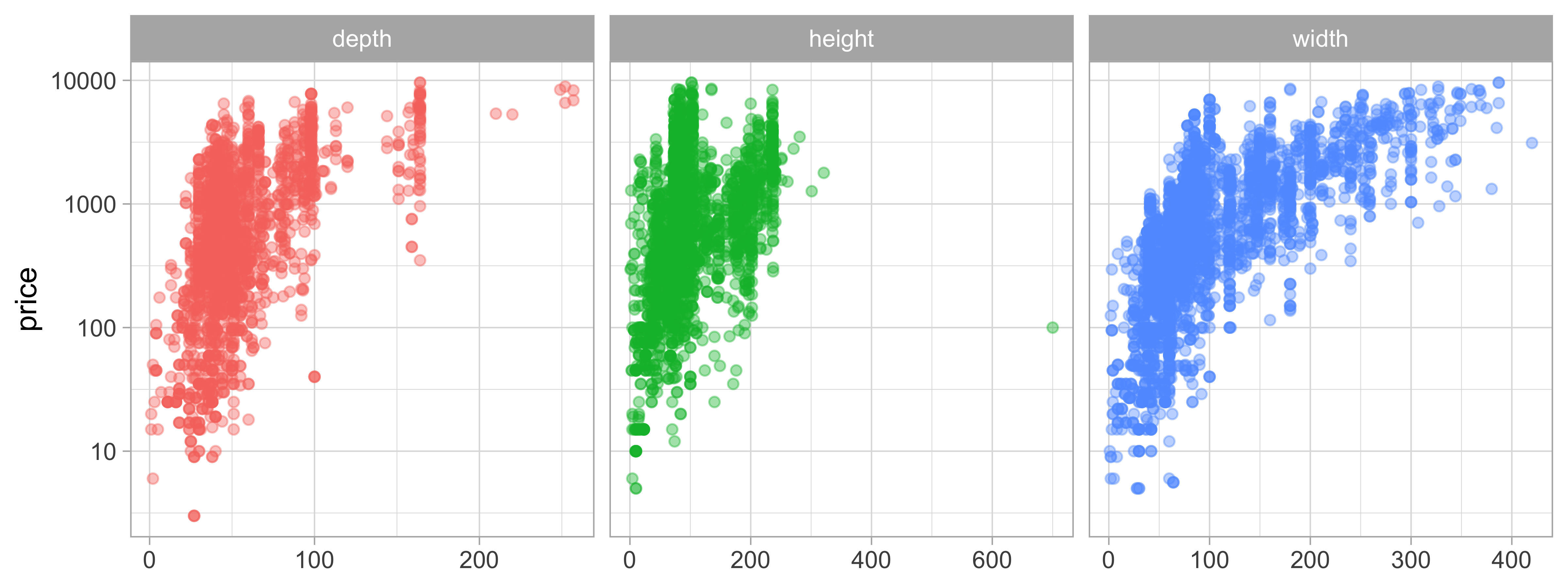
There are lots more great examples of #TidyTuesday EDA out there to explore on Twitter! Let’s do a bit of data preparation for modeling. There are still lots of NA values for furniture dimensions but we are going to impute those.

ikea_df <- ikea %>%
  select(price, name, category, depth, height, width) %>%
  mutate(price = log10(price)) %>%
  mutate_if(is.character, factor)

ikea_df

## # A tibble: 3,694 x 6
##    price name                  category      depth height width
##    <dbl> <fct>                 <fct>         <dbl>  <dbl> <dbl>
##  1  2.42 FREKVENS              Bar furniture    NA     99    51
##  2  3.00 NORDVIKEN             Bar furniture    NA    105    80
##  3  3.32 NORDVIKEN / NORDVIKEN Bar furniture    NA     NA    NA
##  4  1.84 STIG                  Bar furniture    50    100    60
##  5  2.35 NORBERG               Bar furniture    60     43    74
##  6  2.54 INGOLF                Bar furniture    45     91    40
##  7  2.11 FRANKLIN              Bar furniture    44     95    50
##  8  2.29 DALFRED               Bar furniture    50     NA    50
##  9  2.11 FRANKLIN              Bar furniture    44     95    50
## 10  3.34 EKEDALEN / EKEDALEN   Bar furniture    NA     NA    NA
## # … with 3,684 more rows

Build a model

We can start by loading the tidymodels metapackage, splitting our data into training and testing sets, and creating resamples.

library(tidymodels)

set.seed(123)
ikea_split <- initial_split(ikea_df, strata = price)
ikea_train <- training(ikea_split)
ikea_test <- testing(ikea_split)

set.seed(234)
ikea_folds <- bootstraps(ikea_train, strata = price)
ikea_folds

## # Bootstrap sampling using stratification 
## # A tibble: 25 x 2
##    splits             id         
##    <list>             <chr>      
##  1 <split [2.8K/998]> Bootstrap01
##  2 <split [2.8K/1K]>  Bootstrap02
##  3 <split [2.8K/1K]>  Bootstrap03
##  4 <split [2.8K/1K]>  Bootstrap04
##  5 <split [2.8K/1K]>  Bootstrap05
##  6 <split [2.8K/1K]>  Bootstrap06
##  7 <split [2.8K/1K]>  Bootstrap07
##  8 <split [2.8K/1K]>  Bootstrap08
##  9 <split [2.8K/1K]>  Bootstrap09
## 10 <split [2.8K/1K]>  Bootstrap10
## # … with 15 more rows

In this analysis, we are using a function from usemodels to provide scaffolding for getting started with tidymodels tuning. The two inputs we need are:

• a formula to describe our model price ~ .
• our training data ikea_train

library(usemodels)
use_ranger(price ~ ., data = ikea_train)
## lots of options, like use_xgboost, use_glmnet, etc

The output that we get from the usemodels scaffolding sets us up for random forest tuning, and we can add just a few more feature engineering steps to take care of the numerous factor levels in the furniture name and category, “cleaning” the factor levels, and imputing the missing data in the furniture dimensions. Then it’s time to tune!

library(textrecipes)
ranger_recipe <-
  recipe(formula = price ~ ., data = ikea_train) %>%
  step_other(name, category, threshold = 0.01) %>%
  step_clean_levels(name, category) %>%
  step_knnimpute(depth, height, width)

ranger_spec <-
  rand_forest(mtry = tune(), min_n = tune(), trees = 1000) %>%
  set_mode("regression") %>%
  set_engine("ranger")

ranger_workflow <-
  workflow() %>%
  add_recipe(ranger_recipe) %>%
  add_model(ranger_spec)

set.seed(8577)
doParallel::registerDoParallel()
ranger_tune <-
  tune_grid(ranger_workflow,
    resamples = ikea_folds,
    grid = 11
  )

The usemodels output required us to decide for ourselves on the resamples and grid to use; it provides sensible defaults for many options based on our data but we still need to use good judgment for some modeling inputs.

Explore results

Now let’s see how we did. We can check out the best-performing models in the tuning results.

show_best(ranger_tune, metric = "rmse")

## # A tibble: 5 x 8
##    mtry min_n .metric .estimator  mean     n std_err .config              
##   <int> <int> <chr>   <chr>      <dbl> <int>   <dbl> <chr>                
## 1     2     4 rmse    standard   0.342    25 0.00211 Preprocessor1_Model10
## 2     4    10 rmse    standard   0.348    25 0.00234 Preprocessor1_Model05
## 3     5     6 rmse    standard   0.349    25 0.00267 Preprocessor1_Model06
## 4     3    18 rmse    standard   0.351    25 0.00211 Preprocessor1_Model01
## 5     2    21 rmse    standard   0.355    25 0.00197 Preprocessor1_Model08

show_best(ranger_tune, metric = "rsq")

## # A tibble: 5 x 8
##    mtry min_n .metric .estimator  mean     n std_err .config              
##   <int> <int> <chr>   <chr>      <dbl> <int>   <dbl> <chr>                
## 1     2     4 rsq     standard   0.714    25 0.00336 Preprocessor1_Model10
## 2     4    10 rsq     standard   0.704    25 0.00367 Preprocessor1_Model05
## 3     5     6 rsq     standard   0.703    25 0.00408 Preprocessor1_Model06
## 4     3    18 rsq     standard   0.698    25 0.00336 Preprocessor1_Model01
## 5     2    21 rsq     standard   0.694    25 0.00324 Preprocessor1_Model08

How did all the possible parameter combinations do?

autoplot(ranger_tune)

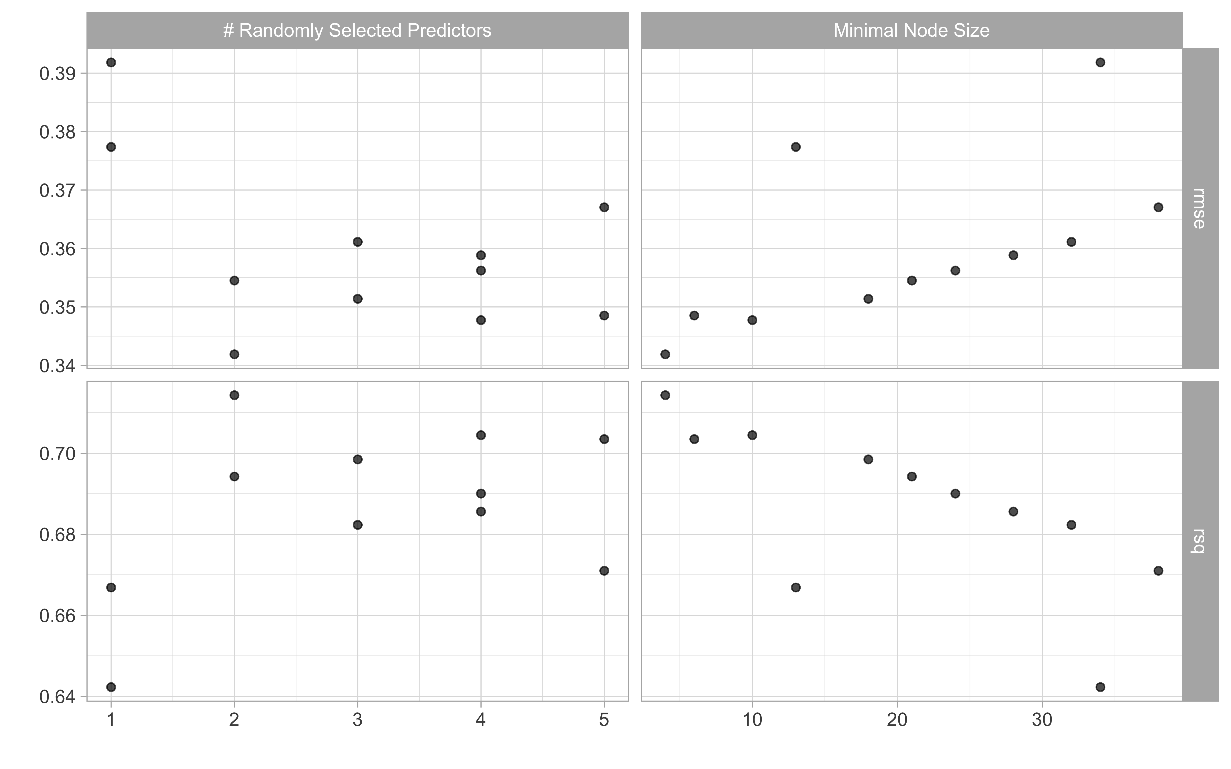
We can finalize our random forest workflow with the best performing parameters.

final_rf <- ranger_workflow %>%
  finalize_workflow(select_best(ranger_tune))

final_rf

## ══ Workflow ════════════════════════════════════════════════════════════════════
## Preprocessor: Recipe
## Model: rand_forest()
## 
## ── Preprocessor ────────────────────────────────────────────────────────────────
## 3 Recipe Steps
## 
## ● step_other()
## ● step_clean_levels()
## ● step_knnimpute()
## 
## ── Model ───────────────────────────────────────────────────────────────────────
## Random Forest Model Specification (regression)
## 
## Main Arguments:
##   mtry = 2
##   trees = 1000
##   min_n = 4
## 
## Computational engine: ranger

The function last_fit() fits this finalized random forest one last time to the training data and evaluates one last time on the testing data.

ikea_fit <- last_fit(final_rf, ikea_split)
ikea_fit

## # Resampling results
## # Manual resampling 
## # A tibble: 1 x 6
##   splits        id           .metrics      .notes      .predictions    .workflow
##   <list>        <chr>        <list>        <list>      <list>          <list>   
## 1 <split [2.8K… train/test … <tibble [2 ×… <tibble [0… <tibble [922 ×… <workflo…

The metrics in ikea_fit are computed using the testing data.

collect_metrics(ikea_fit)

## # A tibble: 2 x 4
##   .metric .estimator .estimate .config             
##   <chr>   <chr>          <dbl> <chr>               
## 1 rmse    standard       0.314 Preprocessor1_Model1
## 2 rsq     standard       0.769 Preprocessor1_Model1

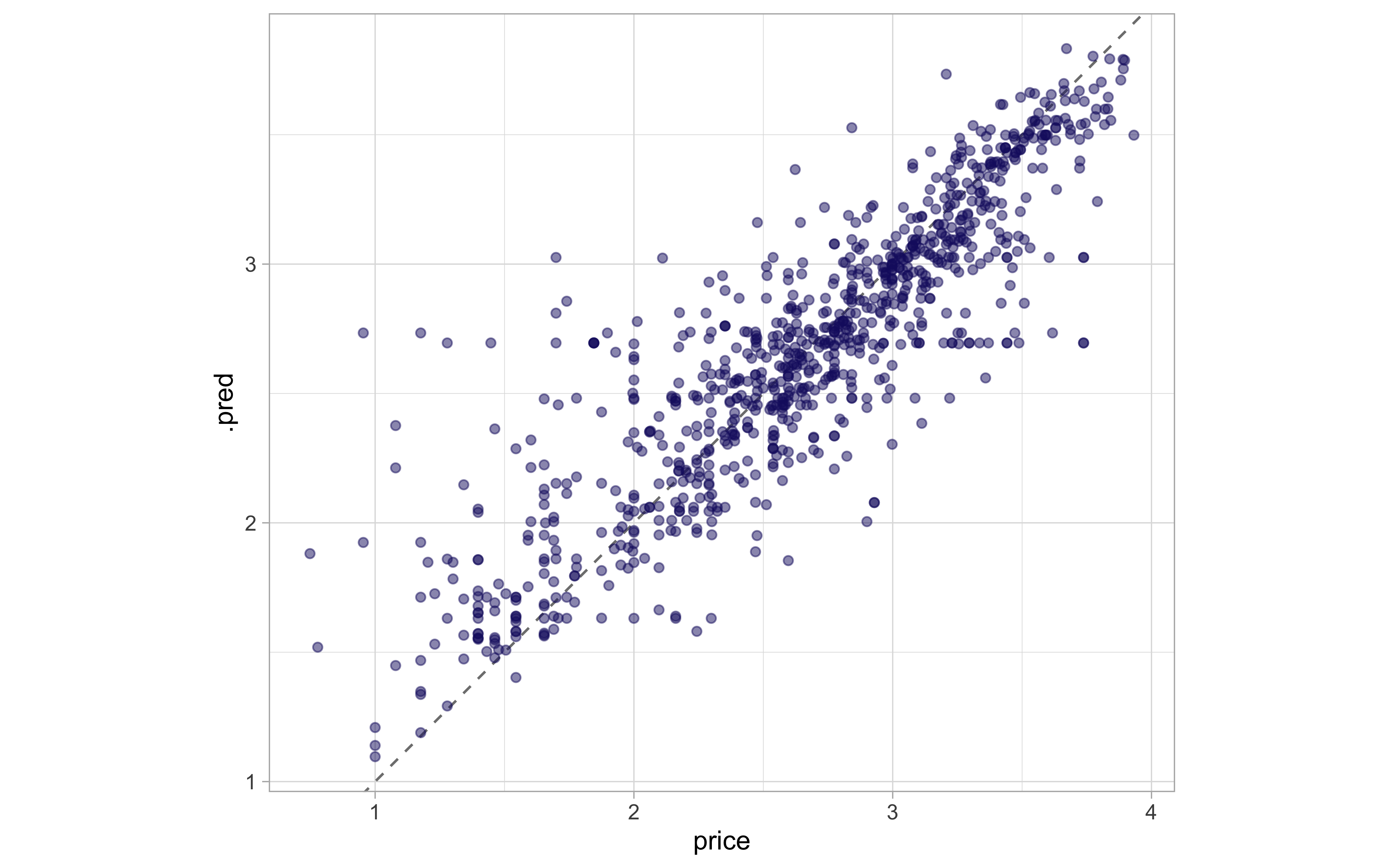
The predictions in ikea_fit are also for the testing data.

collect_predictions(ikea_fit) %>%
  ggplot(aes(price, .pred)) +
  geom_abline(lty = 2, color = "gray50") +
  geom_point(alpha = 0.5, color = "midnightblue") +
  coord_fixed()

We can use the trained workflow from ikea_fit for prediction, or save it to use later.

predict(ikea_fit$.workflow[[1]], ikea_test[15, ])

## # A tibble: 1 x 1
##   .pred
##   <dbl>
## 1  2.72

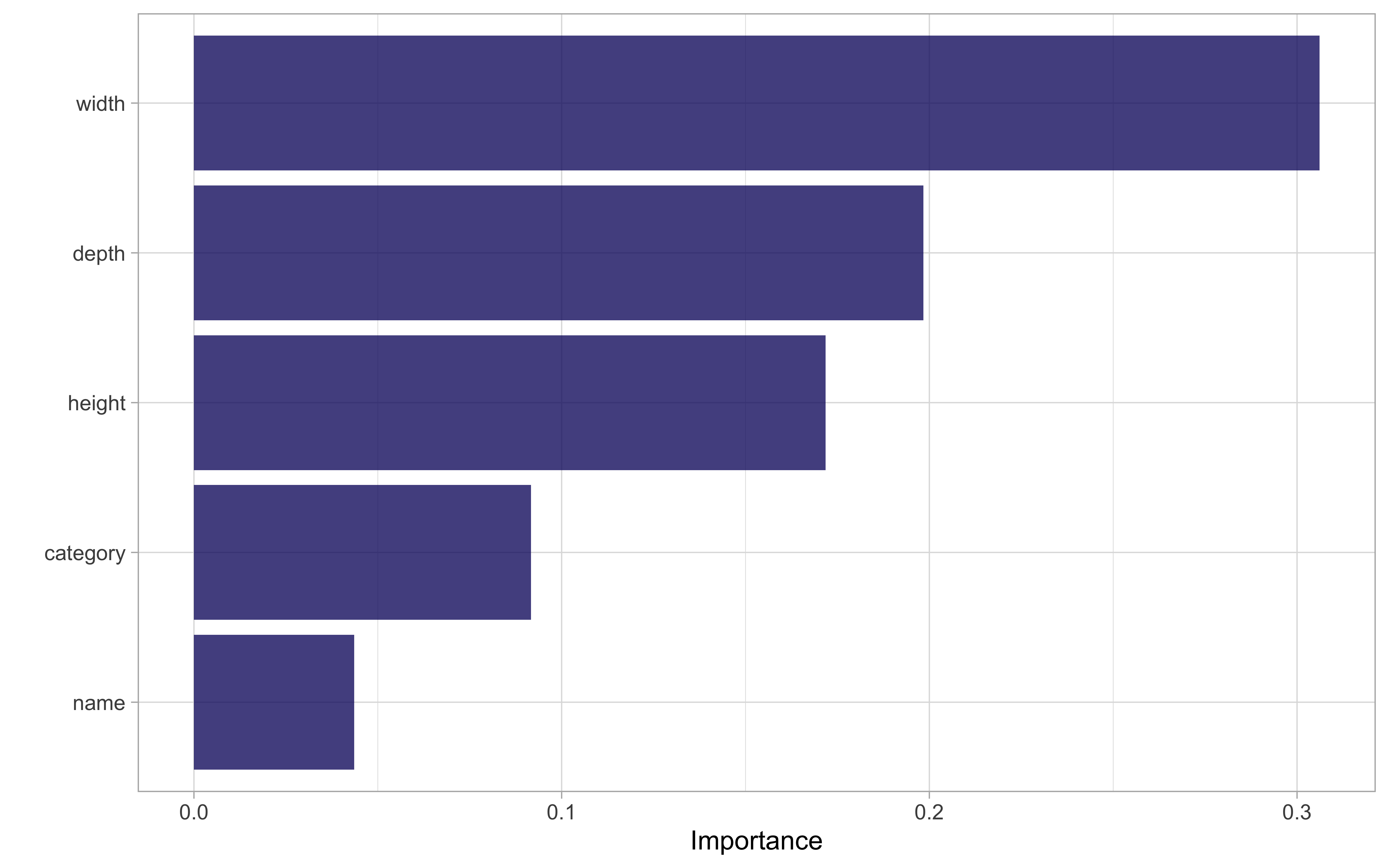
Lastly, let’s learn about feature importance for this model using the vip package. For a ranger model, we do need to go back to the model specification itself and update the engine with importance = "permutation" in order to compute feature importance. This means fitting the model one more time.

library(vip)

imp_spec <- ranger_spec %>%
  finalize_model(select_best(ranger_tune)) %>%
  set_engine("ranger", importance = "permutation")

workflow() %>%
  add_recipe(ranger_recipe) %>%
  add_model(imp_spec) %>%
  fit(ikea_train) %>%
  pull_workflow_fit() %>%
  vip(aesthetics = list(alpha = 0.8, fill = "midnightblue"))