Build a #TidyTuesday predictive text model for The Last Airbender

Lately I’ve been publishing screencasts demonstrating how to use the tidymodels framework, from first steps in modeling to how to evaluate complex models. Today’s screencast admittedly does not result in the best performing model you’ll ever see, but it is really fun and uses this week’s #TidyTuesday dataset on Avatar: The Last Airbender. 🔥 🌏 🌊 💨

Here is the code I used in the video, for those who prefer reading instead of or in addition to video.

Explore the data

This week’s #TidyTuesday dataset is from episodes of Avatar: The Last Airbender, which is a popular show at my house for sure! Our modeling goal is to predict the speaker of each line of dialogue.

library(tidyverse)
avatar_raw <- read_csv("https://raw.githubusercontent.com/rfordatascience/tidytuesday/master/data/2020/2020-08-11/avatar.csv")

avatar_raw %>%
  count(character, sort = TRUE)

## # A tibble: 374 x 2
##    character             n
##    <chr>             <int>
##  1 Scene Description  3393
##  2 Aang               1796
##  3 Sokka              1639
##  4 Katara             1437
##  5 Zuko                776
##  6 Toph                507
##  7 Iroh                337
##  8 Azula               211
##  9 Jet                 134
## 10 Suki                114
## # … with 364 more rows

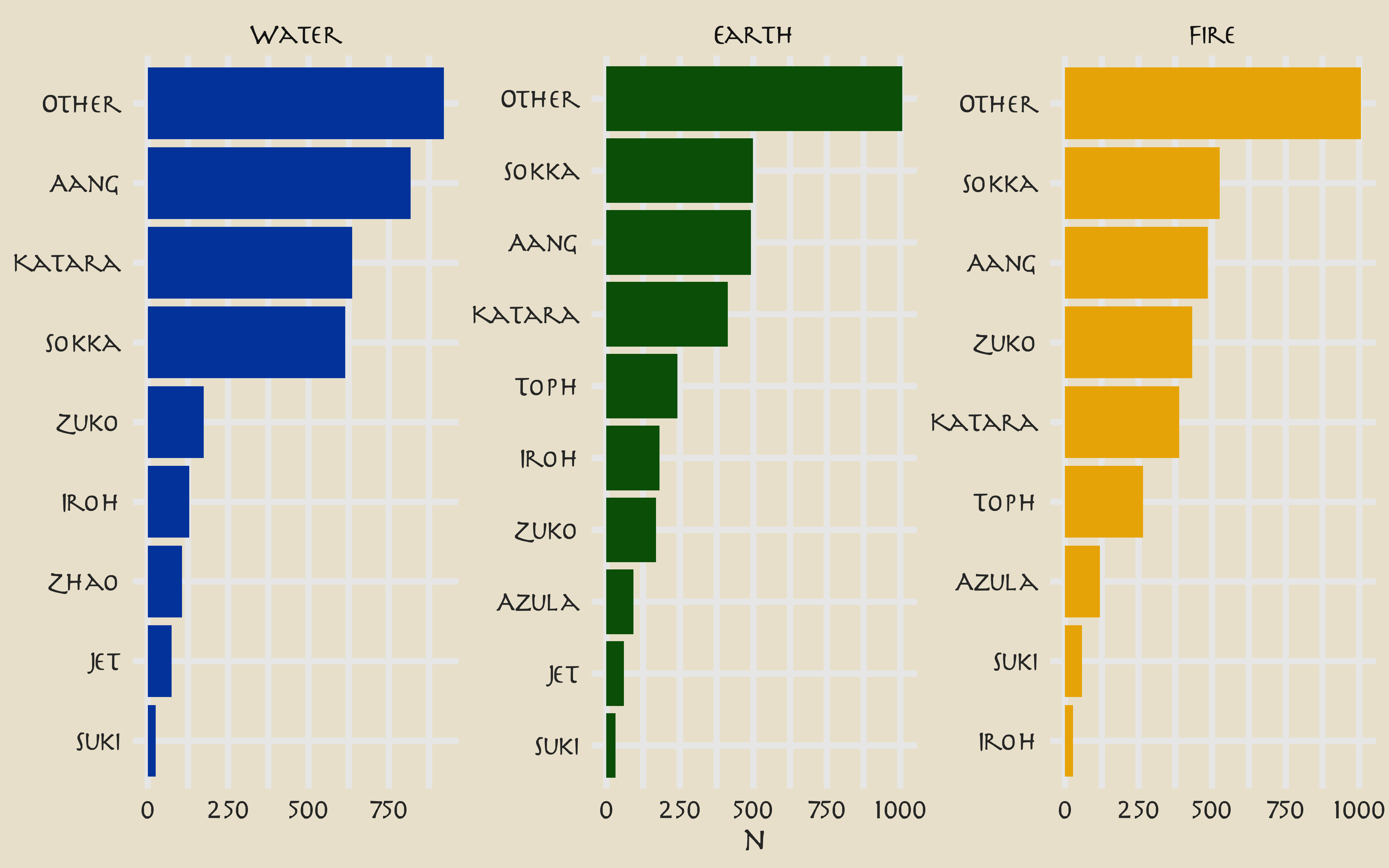
Rows with Scene Description are not dialogue; the main character Aang speaks the most lines overall. How does this change through the three “books” of the show?

library(tidytext)

avatar_raw %>%
  filter(!is.na(character_words)) %>%
  mutate(
    book = fct_inorder(book),
    character = fct_lump_n(character, 10)
  ) %>%
  count(book, character) %>%
  mutate(character = reorder_within(character, n, book)) %>%
  ggplot(aes(n, character, fill = book)) +
  geom_col(show.legend = FALSE) +
  facet_wrap(~book, scales = "free") +
  scale_y_reordered() +
  scale_fill_manual(values = c(
    avatar_pal("WaterTribe")(1),
    avatar_pal("EarthKingdom")(1),
    avatar_pal("FireNation")(1)
  )) +
  labs(y = NULL)

Let’s create a dataset for our modeling question, and look at a few example lines.

avatar <- avatar_raw %>%
  filter(!is.na(character_words)) %>%
  mutate(aang = if_else(character == "Aang", "Aang", "Other")) %>%
  select(aang, book, text = character_words)

avatar %>%
  filter(aang == "Aang") %>%
  sample_n(10) %>%
  pull(text)

##  [1] "What is wrong with me ..."                                                        
##  [2] "That was amazing!"                                                                
##  [3] "Sokka! Are you okay?"                                                             
##  [4] "I thought about what you said, I promise I'll be more patient."                   
##  [5] "If we're going to be here for a month, we should spend our time looking for Appa."
##  [6] "I wish I knew how to make a hurricane!"                                           
##  [7] "But what about expressing yourself?"                                              
##  [8] "What does that even mean?"                                                        
##  [9] "It's from the Eastern Air Temple."                                                
## [10] "Look what I brought to this place."

This… may be a challenge.

What are the highest log odds words from Aang and other speakers?

library(tidytext)
library(tidylo)

avatar_lo <- avatar %>%
  unnest_tokens(word, text) %>%
  count(aang, word) %>%
  bind_log_odds(aang, word, n) %>%
  arrange(-log_odds_weighted)

avatar_lo %>%
  group_by(aang) %>%
  top_n(15) %>%
  ungroup() %>%
  mutate(word = reorder(word, log_odds_weighted)) %>%
  ggplot(aes(log_odds_weighted, word, fill = aang)) +
  geom_col(alpha = 0.8, show.legend = FALSE) +
  facet_wrap(~aang, scales = "free") +
  scale_fill_avatar(palette = "AirNomads") +
  labs(y = NULL)

These words make sense, but the counts are probably too low to build a good model with. Instead, let’s try using text features like the number of punctuation characters, number of pronons, and so forth.

library(textfeatures)

tf <- textfeatures(
  avatar,
  sentiment = FALSE, word_dims = 0,
  normalize = FALSE, verbose = FALSE
)

tf %>%
  bind_cols(avatar) %>%
  group_by(aang) %>%
  summarise(across(starts_with("n_"), mean)) %>%
  pivot_longer(starts_with("n_"), names_to = "text_feature") %>%
  filter(value > 0.01) %>%
  mutate(text_feature = fct_reorder(text_feature, -value)) %>%
  ggplot(aes(aang, value, fill = aang)) +
  geom_col(position = "dodge", alpha = 0.8, show.legend = FALSE) +
  facet_wrap(~text_feature, scales = "free", ncol = 6) +
  scale_fill_avatar("AirNomads") +
  labs(x = NULL, y = "Mean text features per spoken line")

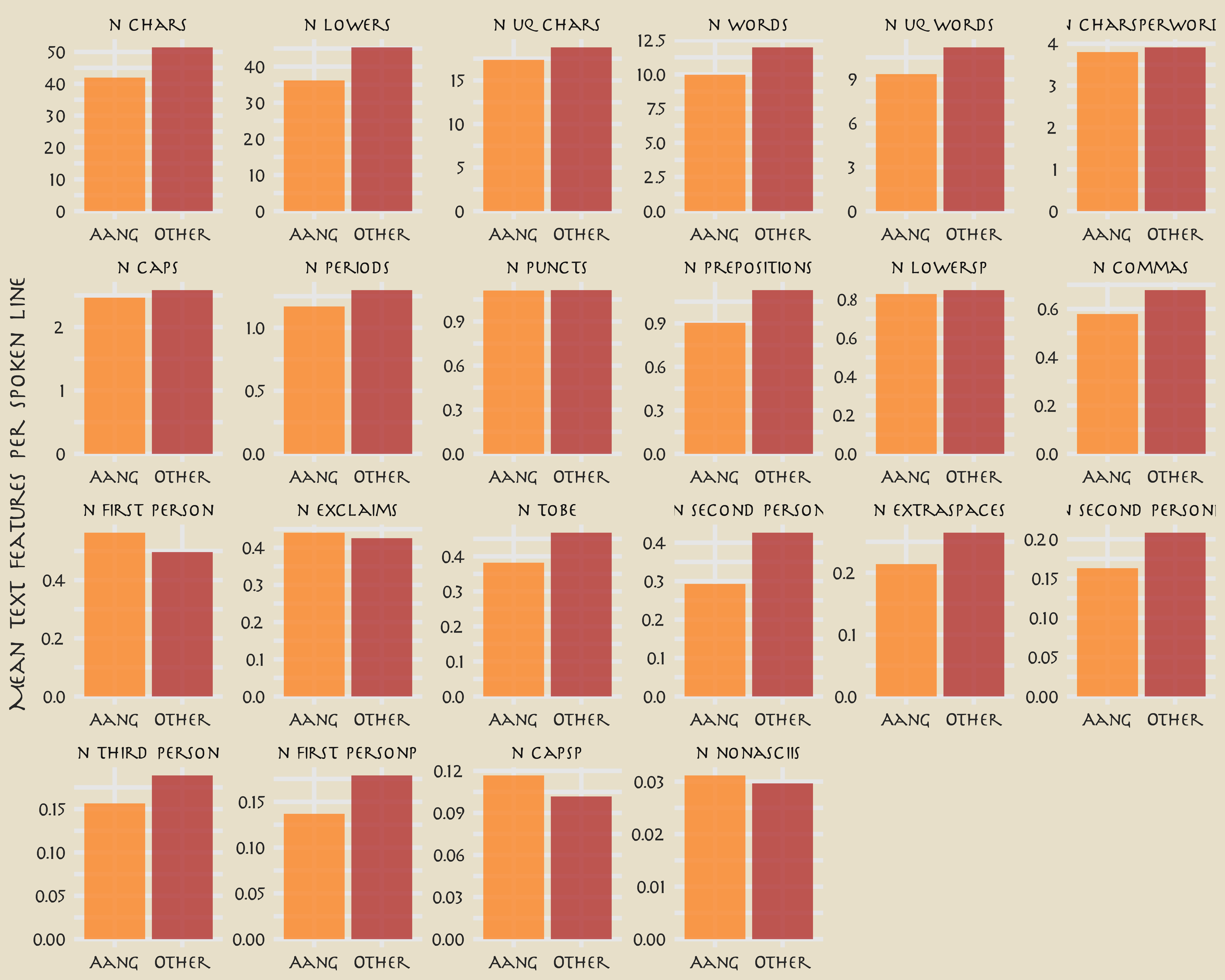
You can read the definitions of these counts here. The differences in these features are what we want to build a model to use in prediction.

Build a model

We can start by loading the tidymodels metapackage, and splitting our data into training and testing sets.

library(tidymodels)

set.seed(123)
avatar_split <- initial_split(avatar, strata = aang)
avatar_train <- training(avatar_split)
avatar_test <- testing(avatar_split)

Next, let’s create cross-validation resamples of the training data, to evaluate our models.

set.seed(234)
avatar_folds <- vfold_cv(avatar_train, strata = aang)
avatar_folds

## #  10-fold cross-validation using stratification 
## # A tibble: 10 x 2
##    splits             id    
##    <list>             <chr> 
##  1 <split [6.7K/750]> Fold01
##  2 <split [6.7K/750]> Fold02
##  3 <split [6.7K/750]> Fold03
##  4 <split [6.7K/750]> Fold04
##  5 <split [6.7K/750]> Fold05
##  6 <split [6.7K/750]> Fold06
##  7 <split [6.7K/750]> Fold07
##  8 <split [6.7K/748]> Fold08
##  9 <split [6.7K/748]> Fold09
## 10 <split [6.7K/748]> Fold10

Next, let’s preprocess our data to get it ready for modeling.

library(textrecipes)
library(themis)

avatar_rec <- recipe(aang ~ text, data = avatar_train) %>%
  step_downsample(aang) %>%
  step_textfeature(text) %>%
  step_zv(all_predictors()) %>%
  step_normalize(all_predictors())

avatar_prep <- prep(avatar_rec)
avatar_prep

## Data Recipe
## 
## Inputs:
## 
##       role #variables
##    outcome          1
##  predictor          1
## 
## Training data contained 7494 data points and no missing data.
## 
## Operations:
## 
## Down-sampling based on aang [trained]
## Text feature extraction for text [trained]
## Zero variance filter removed 14 items [trained]
## Centering and scaling for 13 items [trained]

juice(avatar_prep)

## # A tibble: 2,694 x 14
##    aang  textfeature_tex… textfeature_tex… textfeature_tex…
##    <fct>            <dbl>            <dbl>            <dbl>
##  1 Aang            -0.363           -0.358         -0.471  
##  2 Aang            -0.645           -0.694         -0.582  
##  3 Aang            -0.363           -0.358         -0.337  
##  4 Aang            -0.645           -0.694         -0.626  
##  5 Aang            -0.645           -0.694         -0.715  
##  6 Aang            -0.269           -0.246         -0.293  
##  7 Aang            -0.645           -0.694         -0.648  
##  8 Aang             0.107            0.202          0.0849 
##  9 Aang            -0.833           -0.918         -0.870  
## 10 Aang            -0.175           -0.134         -0.00397
## # … with 2,684 more rows, and 10 more variables:
## #   textfeature_text_n_uq_charS <dbl>,
## #   textfeature_text_n_digits <dbl>, textfeature_text_n_commas <dbl>,
## #   textfeature_text_n_periods <dbl>,
## #   textfeature_text_n_exclaims <dbl>,
## #   textfeature_text_n_extraspaces <dbl>,
## #   textfeature_text_n_caps <dbl>, textfeature_text_n_lowers <dbl>,
## #   textfeature_text_n_nonasciis <dbl>,
## #   textfeature_text_n_puncts <dbl>

Let’s walk through the steps in this recipe.

• First, we must tell the recipe() what our model is going to be (using a formula here) and what data we are using.
• Next, we downsample for our predictor, since there are many more lines spoken by characters other than Aang than by Aang.
• We create the text features using a step from the textrecipes package.
• Then we remove zero-variance variables, which includes variables like the text features about URLs and hashtags in this case.
• Finally, we center and scale the predictors because of the specific kind of model we want to try out.

We’re mostly going to use this recipe in a workflow() so we don’t need to stress too much about whether to prep() or not. Since we are going to compute variable importance, we will need to come back to juice(avatar_prep).

Let’s compare two different models, a random forest model and a support vector machine model. We start by creating the model specifications.

rf_spec <- rand_forest(trees = 1000) %>%
  set_engine("ranger") %>%
  set_mode("classification")

rf_spec

## Random Forest Model Specification (classification)
## 
## Main Arguments:
##   trees = 1000
## 
## Computational engine: ranger

svm_spec <- svm_rbf(cost = 0.5) %>%
  set_engine("kernlab") %>%
  set_mode("classification")

svm_spec

## Radial Basis Function Support Vector Machine Specification (classification)
## 
## Main Arguments:
##   cost = 0.5
## 
## Computational engine: kernlab

Next let’s start putting together a tidymodels workflow(), a helper object to help manage modeling pipelines with pieces that fit together like Lego blocks. Notice that there is no model yet: Model: None.

avatar_wf <- workflow() %>%
  add_recipe(avatar_rec)

avatar_wf

## ══ Workflow ══════════════════════════════════════════════════════════
## Preprocessor: Recipe
## Model: None
## 
## ── Preprocessor ──────────────────────────────────────────────────────
## 4 Recipe Steps
## 
## ● step_downsample()
## ● step_textfeature()
## ● step_zv()
## ● step_normalize()

Now we can add a model, and the fit to each of the resamples. First, we can fit the random forest model.

doParallel::registerDoParallel()

set.seed(1234)
rf_rs <- avatar_wf %>%
  add_model(rf_spec) %>%
  fit_resamples(
    resamples = avatar_folds,
    metrics = metric_set(roc_auc, accuracy, sens, spec),
    control = control_grid(save_pred = TRUE)
  )

Second, we can fit the support vector machine model.

set.seed(2345)
svm_rs <- avatar_wf %>%
  add_model(svm_spec) %>%
  fit_resamples(
    resamples = avatar_folds,
    metrics = metric_set(roc_auc, accuracy, sens, spec),
    control = control_grid(save_pred = TRUE)
  )

We have fit each of our candidate models to our resampled training set!

Evaluate model

It’s time to see how we did.

collect_metrics(rf_rs)

## # A tibble: 4 x 5
##   .metric  .estimator  mean     n std_err
##   <chr>    <chr>      <dbl> <int>   <dbl>
## 1 accuracy binary     0.525    10 0.00536
## 2 roc_auc  binary     0.541    10 0.00809
## 3 sens     binary     0.540    10 0.0104 
## 4 spec     binary     0.522    10 0.00632

conf_mat_resampled(rf_rs)

## # A tibble: 4 x 3
##   Prediction Truth  Freq
##   <fct>      <fct> <dbl>
## 1 Aang       Aang   72.8
## 2 Aang       Other 294. 
## 3 Other      Aang   61.9
## 4 Other      Other 321.

Well, that is underwhelming!

collect_metrics(svm_rs)

## # A tibble: 4 x 5
##   .metric  .estimator  mean     n std_err
##   <chr>    <chr>      <dbl> <int>   <dbl>
## 1 accuracy binary     0.514    10 0.00885
## 2 roc_auc  binary     0.556    10 0.00744
## 3 sens     binary     0.585    10 0.0183 
## 4 spec     binary     0.498    10 0.0133

conf_mat_resampled(svm_rs)

## # A tibble: 4 x 3
##   Prediction Truth  Freq
##   <fct>      <fct> <dbl>
## 1 Aang       Aang   78.8
## 2 Aang       Other 308. 
## 3 Other      Aang   55.9
## 4 Other      Other 306.

Different, but not really better! The SVM model is better able to identify the positive cases but at the expense of the negative cases. Overall, we definitely see that this is a hard problem that we barely are able to have any predictive ability for.

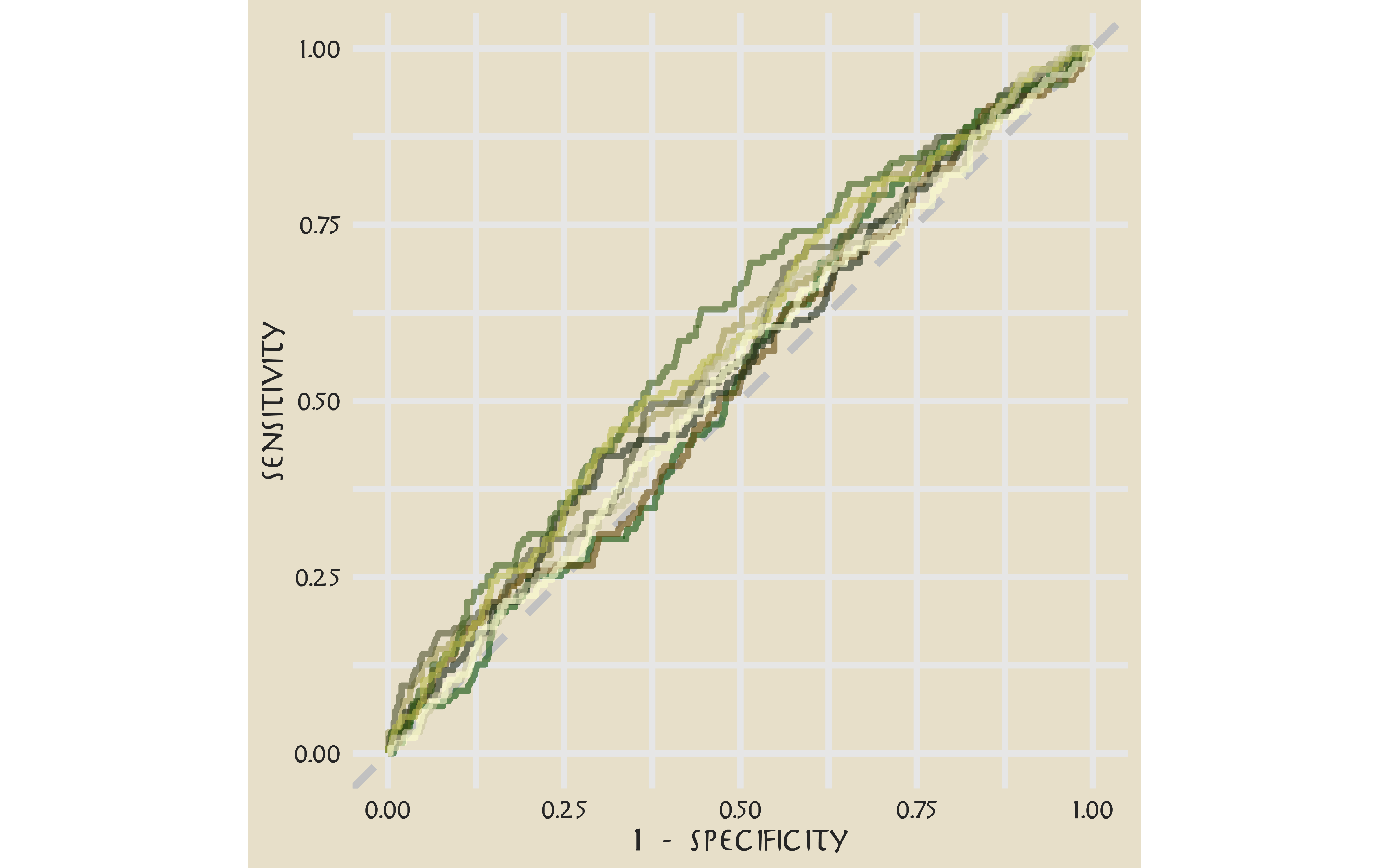
Let’s say we are more interested in detecting Aang’s lines, even at the expense of the false positives.

svm_rs %>%
  collect_predictions() %>%
  group_by(id) %>%
  roc_curve(aang, .pred_Aang) %>%
  ggplot(aes(1 - specificity, sensitivity, color = id)) +
  geom_abline(lty = 2, color = "gray80", size = 1.5) +
  geom_path(show.legend = FALSE, alpha = 0.6, size = 1.2) +
  scale_color_avatar(palette = "EarthKingdom") +
  coord_equal()

This plot highlights how this model is barely doing better than guessing.

Keeping in mind the realities of our model performance, let’s talk about how to compute variable importance for a model like an SVM, which does not have information within it about variable importance like a linear model or a tree-based model. In this case, we can use a method like permutation of the variables.

library(vip)

set.seed(345)
avatar_imp <- avatar_wf %>%
  add_model(svm_spec) %>%
  fit(avatar_train) %>%
  pull_workflow_fit() %>%
  vi(
    method = "permute", nsim = 10,
    target = "aang", metric = "auc", reference_class = "Other",
    pred_wrapper = kernlab::predict, train = juice(avatar_prep)
  )

avatar_imp %>%
  slice_max(Importance, n = 8) %>%
  mutate(
    Variable = str_remove(Variable, "textfeature_text_n_"),
    Variable = fct_reorder(Variable, Importance)
  ) %>%
  ggplot(aes(Importance, Variable, color = Variable)) +
  geom_errorbar(aes(xmin = Importance - StDev, xmax = Importance + StDev),
    alpha = 0.5, size = 1.3
  ) +
  geom_point(size = 3) +
  theme(legend.position = "none") +
  scale_color_avatar(palette = "FireNation") +
  labs(y = NULL)

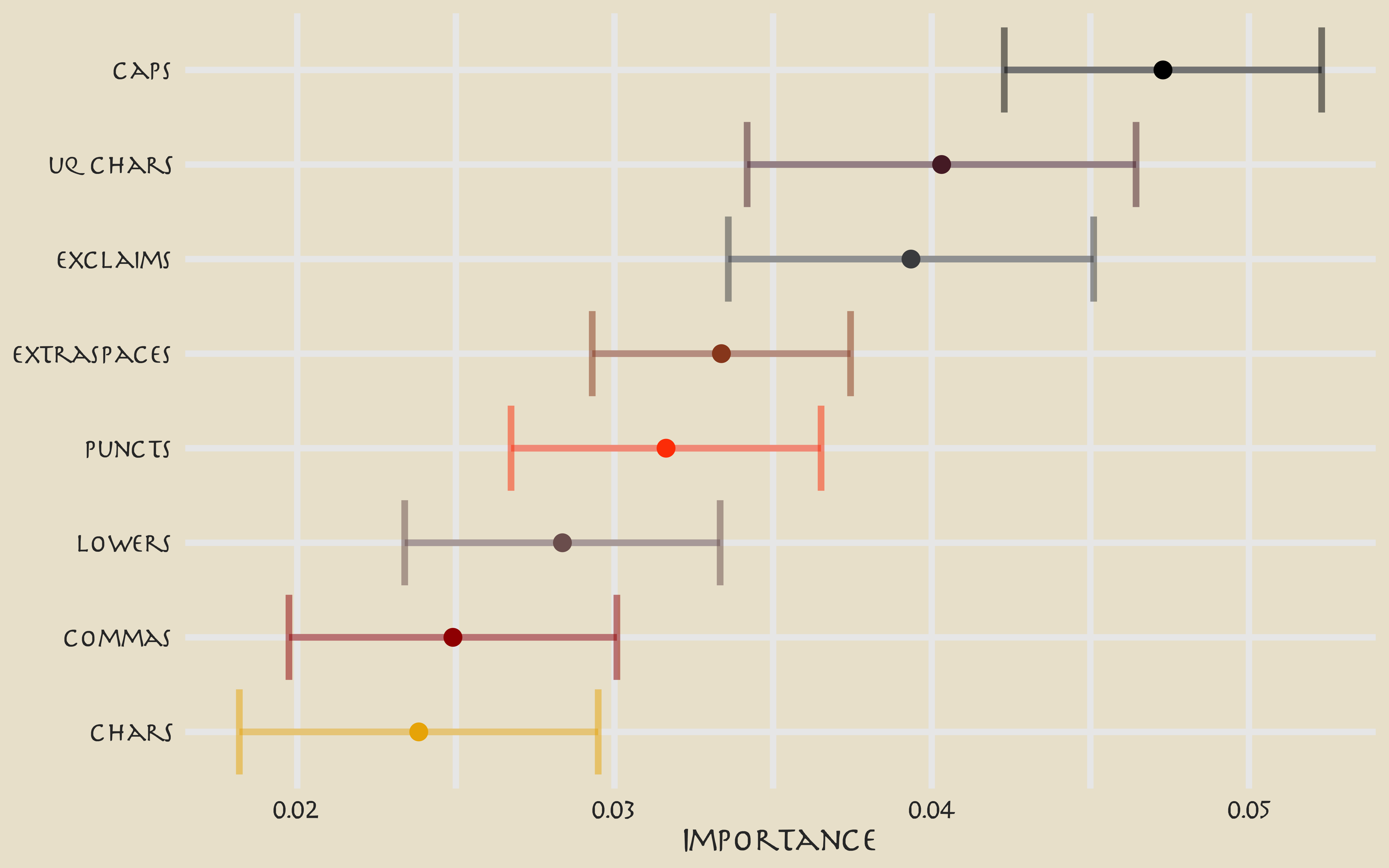
These are the text features that are most important globally for whether a line was spoken by Aang or not.

Finally, we can return to the testing data to confirm that our (admittedly lackluster) performance is about the same.

avatar_final <- avatar_wf %>%
  add_model(svm_spec) %>%
  last_fit(avatar_split)

avatar_final %>%
  collect_metrics()

## # A tibble: 2 x 3
##   .metric  .estimator .estimate
##   <chr>    <chr>          <dbl>
## 1 accuracy binary         0.525
## 2 roc_auc  binary         0.557

avatar_final %>%
  collect_predictions() %>%
  conf_mat(aang, .pred_class)

##           Truth
## Prediction Aang Other
##      Aang   243   981
##      Other  206  1068