Spatial resampling for #TidyTuesday and the #30DayMapChallenge

This is the latest in my series of screencasts demonstrating how to use the tidymodels packages, from just getting started to tuning more complex models. Today’s screencast walks through how to use spatial resampling for evaluating a model, with this week’s #TidyTuesday dataset on geographic data. 🗾

Here is the code I used in the video, for those who prefer reading instead of or in addition to video.

Explore data

Geographic data is special when it comes to, well, basically everything! This includes modeling and especially evaluating models. This week’s #TidyTuesday is all about exploring spatial data for the #30DayMapChallenge this month, and especially the spData and spDataLarge packages along with the book Geocomputation with R.

Let’s use the dataset of landslides (plus not-landslide locations) in Southern Ecuador.

data("lsl", package = "spDataLarge")
landslides <- as_tibble(lsl)
landslides

## # A tibble: 350 × 8
##          x        y lslpts slope    cplan     cprof  elev log10_carea
##      <dbl>    <dbl> <fct>  <dbl>    <dbl>     <dbl> <dbl>       <dbl>
##  1 715078. 9558647. FALSE   37.4  0.0205   0.00866  2477.        2.61
##  2 713748. 9558047. FALSE   41.7 -0.0241   0.00679  2486.        3.07
##  3 712508. 9558887. FALSE   20.0  0.0390   0.0147   2142.        2.29
##  4 713998. 9558187. FALSE   45.8 -0.00632  0.00435  2391.        3.83
##  5 714308. 9557307. FALSE   41.7  0.0423  -0.0202   2570.        2.70
##  6 713488. 9558117. FALSE   52.9  0.0323   0.00703  2418.        2.48
##  7 714948. 9558347. FALSE   51.9  0.0399   0.000791 2546.        3.15
##  8 714678. 9560357. FALSE   38.5  0.0164   0.0299   1932.        3.26
##  9 714368. 9560287. FALSE   24.1 -0.0188  -0.00956  2059.        3.20
## 10 712528. 9559217. FALSE   50.5  0.0142   0.0151   1973.        2.60
## # … with 340 more rows

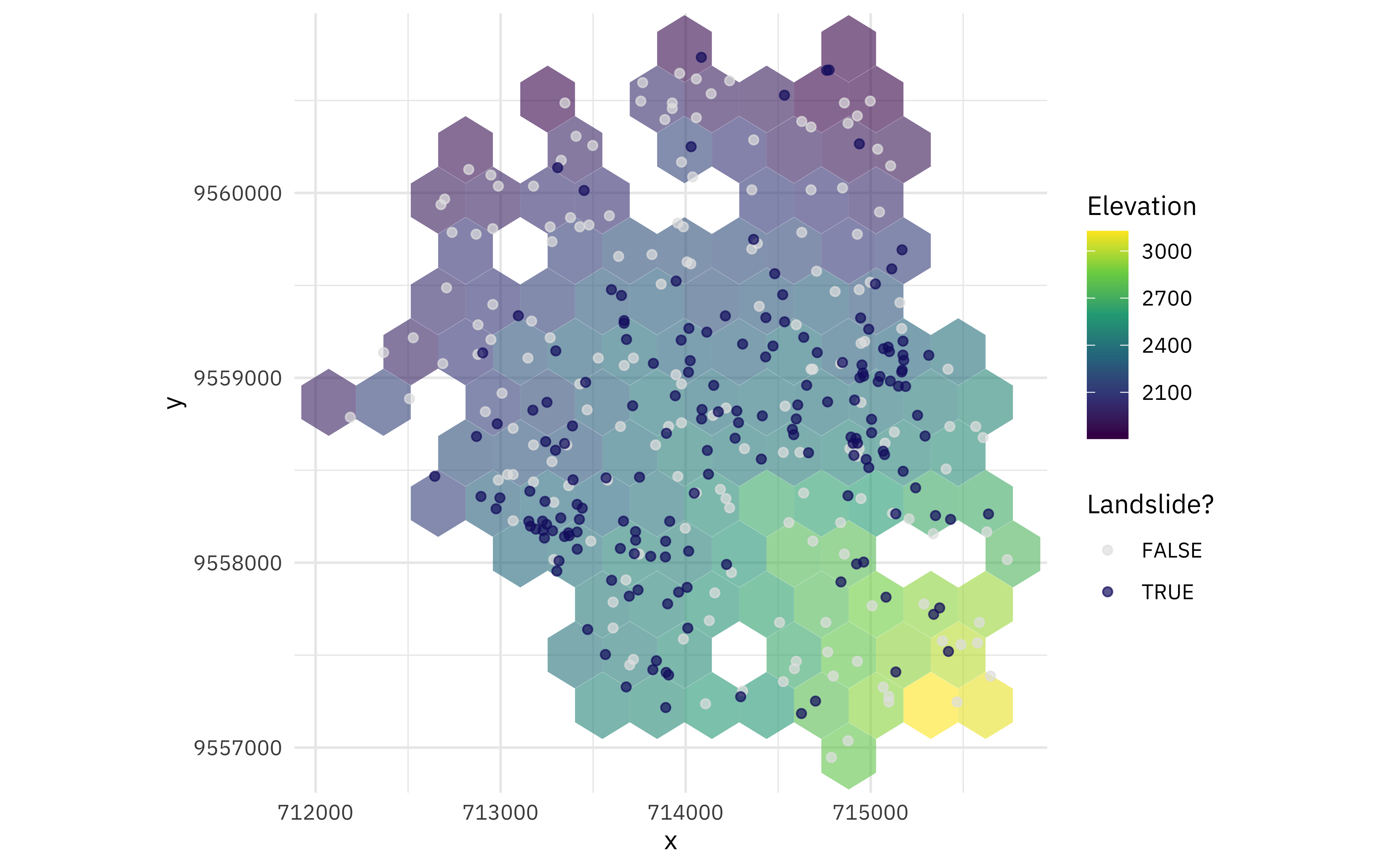
How are these landslides (plus not landslides) distributes in this area?

ggplot(landslides, aes(x, y)) +
  stat_summary_hex(aes(z = elev), alpha = 0.6, bins = 12) +
  geom_point(aes(color = lslpts), alpha = 0.7) +
  coord_fixed() +
  scale_fill_viridis_c() +
  scale_color_manual(values = c("gray90", "midnightblue")) +
  labs(fill = "Elevation", color = "Landslide?")

Create spatial resamples

In tidymodels, one of the first steps we recommend thinking about is “spending your data budget.” When it comes to geographic data, points close to each other are often similar so we don’t want to randomly resample our observations. Instead, we want to use a resampling strategy that accounts for that autocorrelation. Let’s create both resamples that are appropriate to spatial data and resamples that might work for “regular,” non-spatial data but are not a good fit for geographic data.

library(tidymodels)
library(spatialsample)

set.seed(123)
good_folds <- spatial_clustering_cv(landslides, coords = c("x", "y"), v = 5)
good_folds

## #  5-fold spatial cross-validation 
## # A tibble: 5 × 2
##   splits           id   
##   <list>           <chr>
## 1 <split [306/44]> Fold1
## 2 <split [256/94]> Fold2
## 3 <split [251/99]> Fold3
## 4 <split [303/47]> Fold4
## 5 <split [284/66]> Fold5

set.seed(234)
bad_folds <- vfold_cv(landslides, v = 5, strata = lslpts)
bad_folds

## #  5-fold cross-validation using stratification 
## # A tibble: 5 × 2
##   splits           id   
##   <list>           <chr>
## 1 <split [280/70]> Fold1
## 2 <split [280/70]> Fold2
## 3 <split [280/70]> Fold3
## 4 <split [280/70]> Fold4
## 5 <split [280/70]> Fold5

The spatialsample package currently provides one method for spatial resampling and we are interested in hearing about what other methods we should support next.

How do these resamples look? Let’s create a little helper function:

plot_splits <- function(split) {
  p <- bind_rows(
    analysis(split) %>%
      mutate(analysis = "Analysis"),
    assessment(split) %>%
      mutate(analysis = "Assessment")
  ) %>%
    ggplot(aes(x, y, color = analysis)) +
    geom_point(size = 1.5, alpha = 0.8) +
    coord_fixed() +
    labs(color = NULL)
  print(p)
}

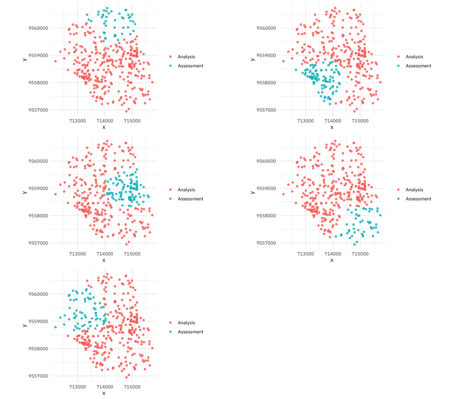
The spatial resampling creates resamples where observations close to each other are together.

walk(good_folds$splits, plot_splits)

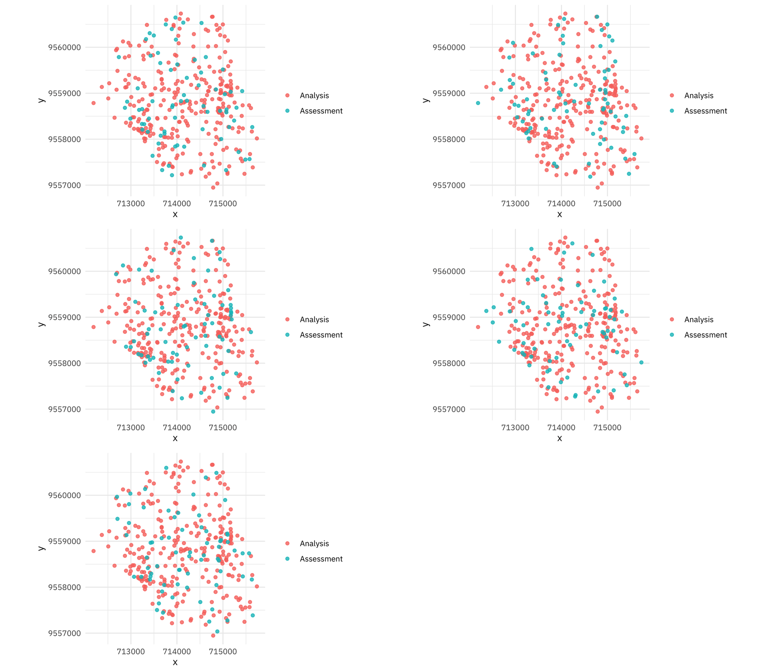
The regular resampling doesn’t do this; it just randomly resamples all observations.

walk(bad_folds$splits, plot_splits)

This second option is not a good idea for geographic data.

Fit and evaluate model

Let’s create a straightforward logistic regression model to predict whether a location saw a landslide based on the other characteristics like slope, elevation, amount of water flow, etc. We can estimate how well this same model fits the data both with our regular folds and our special spatial resampling.

glm_spec <- logistic_reg()
lsl_form <- lslpts ~ slope + cplan + cprof + elev + log10_carea

lsl_wf <- workflow(lsl_form, glm_spec)

doParallel::registerDoParallel()
set.seed(2021)
regular_rs <- fit_resamples(lsl_wf, bad_folds)
set.seed(2021)
spatial_rs <- fit_resamples(lsl_wf, good_folds)

How did our results turn out?

collect_metrics(regular_rs)

## # A tibble: 2 × 6
##   .metric  .estimator  mean     n std_err .config             
##   <chr>    <chr>      <dbl> <int>   <dbl> <chr>               
## 1 accuracy binary     0.737     5  0.0173 Preprocessor1_Model1
## 2 roc_auc  binary     0.808     5  0.0201 Preprocessor1_Model1

collect_metrics(spatial_rs)

## # A tibble: 2 × 6
##   .metric  .estimator  mean     n std_err .config             
##   <chr>    <chr>      <dbl> <int>   <dbl> <chr>               
## 1 accuracy binary     0.677     5 0.0708  Preprocessor1_Model1
## 2 roc_auc  binary     0.782     5 0.00790 Preprocessor1_Model1

If we use the “regular” resampling, we get a more optimistc estimate of performance which would fool us into thinking our model would perform better than it really could. The lower performance estimate using spatial resampling is more accurate because of the autocorrelation of this geographic data; observations near each other are more alike than observations far apart. With geographic data, it’s important to use an appropriate model evaluation strategy!