Return of the NEISS Data

Almost six months ago (!) I wrote a blog post about the NEISS data set, a sample of accidents reported to emergency rooms in the U.S. that are related to consumer products. Ever since I did that exploration, I have been wanting to ask a bit of a different question from that sample of accidents. How do the accidents that people suffer depend on their demographic characteristics? We can get a bit of a sense of that from looking at the plot with age on the x-axis (or exploring Hadley Wickham’s NEISS Shiny app) but the NEISS data set includes quite a bit more demographic information to interact with.

Before we get started, it is probably good to be reminded that this data set doesn’t necessarily include everything you might think it does. After I published that first post, Henrik Bengtsson asked about hang gliding injuries reported in this data set. There appeared to be none, and I was befuddled until Alison Hill pointed out that the NEISS coding manual says that they don’t include such injuries.

@juliasilge @henrikbengtsson yup from here https://t.co/yrDtL27iVx pic.twitter.com/5Dj17ciLQl

— Alison Hill (@apreshill) February 19, 2016

So there you go.

Getting the Data

First, let’s get the NEISS data. It’s a pretty big data set so this can take a while.

library(devtools)
install_github("hadley/neiss")
library(neiss)

Now let’s open up the main data set and see what is there.

data(injuries)
names(injuries)

##  [1] "case_num"    "trmt_date"   "psu"         "weight"      "stratum"    
##  [6] "age"         "sex"         "race"        "race_other"  "diag"       
## [11] "diag_other"  "body_part"   "disposition" "location"    "fmv"        
## [16] "prod1"       "prod2"       "narrative"

Each row is a case, i.e. injury. The consumer product(s) implicated in the injury are in prod1 and prod2 as numbers, which can be looked up in another data set, products. Let’s join these data frames together so we have the product names rather than codes.

library(dplyr)
injuries <- left_join(injuries, products, by = c("prod1" = "code")) %>% 
        rename(product = title)

What Should I Worry About?

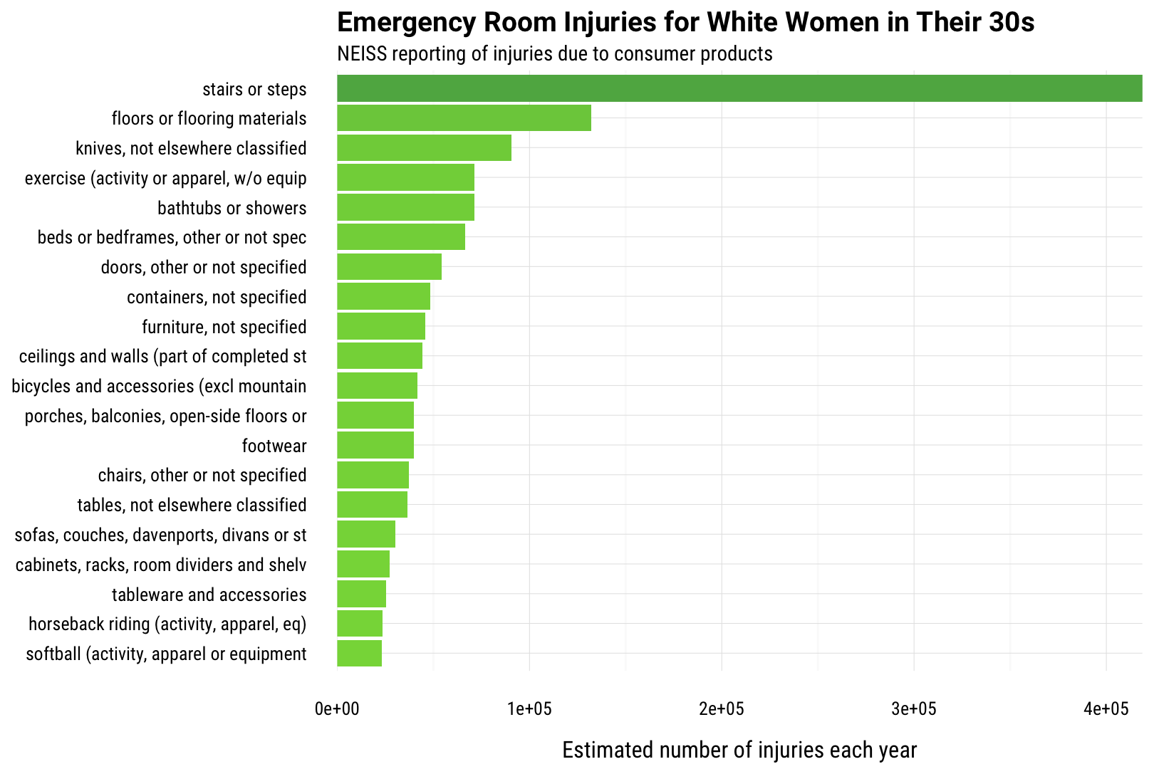
I am a white woman in my (ever later) thirties, so let’s find what the most common injuries are for someone with my demographic characteristics. This is just some basic dplyr.

me <- injuries %>% filter(sex == "Female",
                          race == "White",
                          age >= 30 & age < 40) %>%
        group_by(product) %>%
        summarise(total = sum(weight)) %>% 
        top_n(20, total) %>% arrange(desc(total)) %>%
        mutate(product = factor(product, levels = rev(unique(product))))
me

## # A tibble: 20 x 2
##                                     product     total
##                                      <fctr>     <dbl>
## 1                           stairs or steps 418788.68
## 2              floors or flooring materials 132231.22
## 3          knives, not elsewhere classified  90598.30
## 4  exercise (activity or apparel, w/o equip  71217.00
## 5                       bathtubs or showers  71213.57
## 6      beds or bedframes, other or not spec  66536.09
## 7             doors, other or not specified  54158.15
## 8                 containers, not specified  48236.82
## 9                  furniture, not specified  45926.30
## 10 ceilings and walls (part of completed st  44420.16
## 11  bicycles and accessories (excl mountain  41523.37
## 12  porches, balconies, open-side floors or  39930.77
## 13                                 footwear  39712.56
## 14           chairs, other or not specified  37362.72
## 15         tables, not elsewhere classified  36498.25
## 16 sofas, couches, davenports, divans or st  30144.78
## 17 cabinets, racks, room dividers and shelv  27286.59
## 18                tableware and accessories  25579.41
## 19 horseback riding (activity, apparel, eq)  23512.82
## 20 softball (activity, apparel or equipment  23004.19

Let’s make a visualization for this.

library(ggplot2)
library(ggstance)
library(scales)
ggplot(data = me, aes(x = total, y = product)) + 
        geom_barh(stat="identity", aes(fill = total)) +
        theme_minimal(base_family = "RobotoCondensed-Regular", base_size = 13) +
        theme(plot.title=element_text(family="Roboto-Bold")) +
        theme(legend.position = "none") +
        scale_x_continuous(expand=c(0,0), labels = scientific_format()) +
        scale_fill_gradient(low = "#86d746", high = "#5eb151") +
        labs(y = NULL, x = "Estimated number of injuries each year",
             title = "Emergency Room Injuries for White Women in Their 30s",
             subtitle = "NEISS reporting of injuries due to consumer products") +
        theme(axis.title.x=element_text(margin=margin(t=15)))

Looks like I should really be careful on our basement stairs. (ALSO, KNIVES!!!) There’s still a fair showing for exercise and sports injuries for white women in their (our?) thirties but a lot of this looks very domestic. “Containers, not specified”?! Not sure on that one.

injuries %>% filter(sex == "Female",
                    race == "White",
                    age >= 30 & age < 40,
                    product == "containers, not specified") %>%
        sample_n(5) %>%
        select(narrative)

## # A tibble: 5 x 1
##                                                                          narrative
##                                                                              <chr>
## 1 EXAC. CHRONIC LOW BACK PAIN: 37YOF HAS BEEN MOVING HEAVY BOXES, FELT SOMETHING "
## 2                      A BOX FELL ONTO PT'S SHOULDER. DX:  L SHOULDER CONT/SPRAIN.
## 3 30YOWF  PT REPORTS SHE HELPED MOVE SOME HEAVY BOXES & DEVELOPED L LOWER BACK PAI
## 4                     38YOF-ANKLE INJURY-TWISTED ANKLE WHILE LIFTING A BOX-@ HOME 
## 5 LAC FINGER 33YOF CUTTING OPEN PACKAGE WITH KNIFE CUT FINGER AT HOME DX: LAC FING

So that means boxes mainly, apparently.

What Should YOU Worry About?

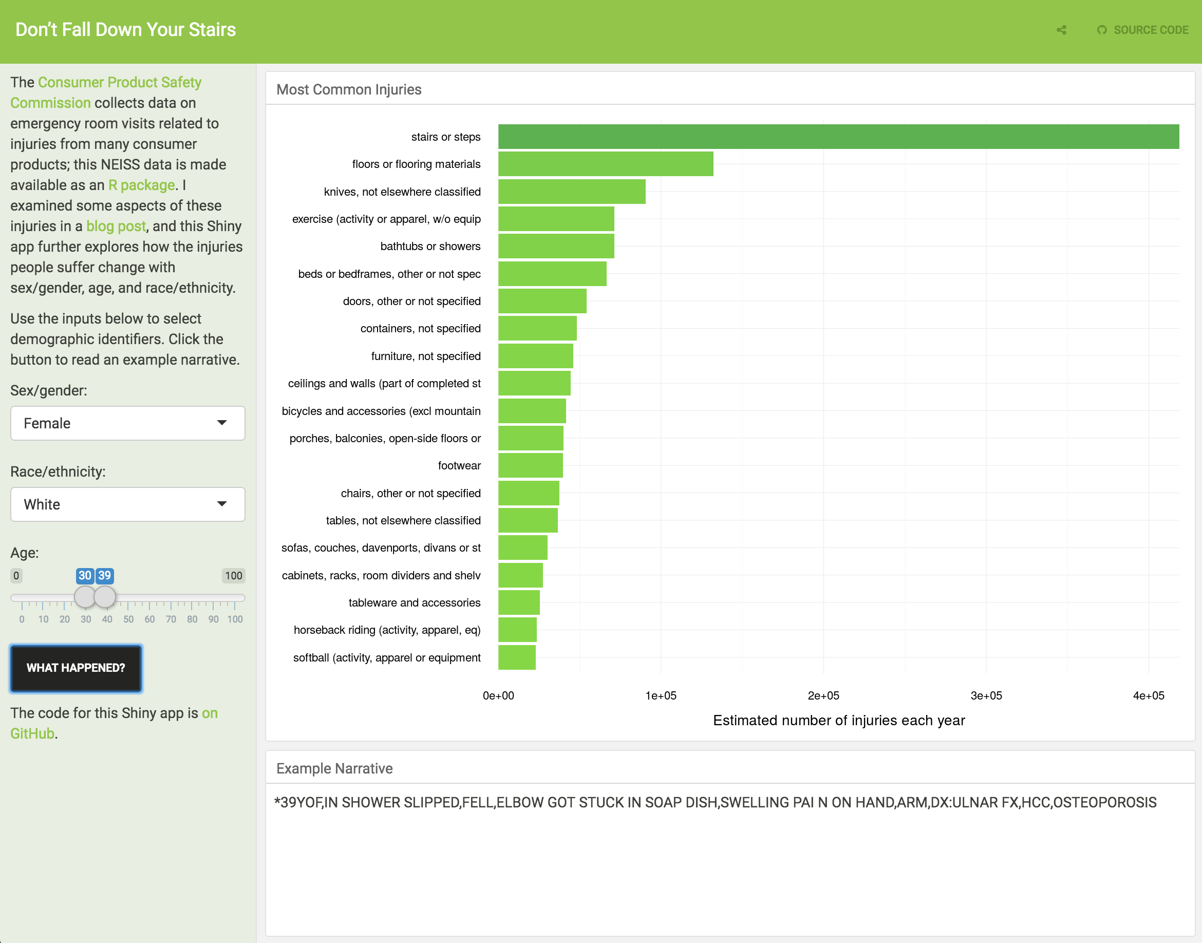
Those are the most common injuries for my demographic, but what about the rest of everyone else? I have made a Shiny app where you can explore the NEISS data and see how the most common injuries change with age, sex, and race/ethnicity. Check out the app itself, and the code to make the app on GitHub.

Race/ethnicity and also sex/gender can be fraught categories for people whose identities are not easily categorizable; I have chosen to just use these demographics as reported. It appears that an age is reported for every injury in the data set (all 2.3 million of them), but there is missing information for sex and race/ethnicity.

mean(injuries$sex == "None listed")

## [1] 3.814901e-05

mean(injuries$race == "None listed")

## [1] 0.2754251

You can look in the Shiny app at the injuries for which these quantities are not reported as “None listed”.

The End

The distribution of common injuries changes quite a lot with various demographic indicators. Check out, for example, the shape of the distribution for children of some sex/race compared to basically any decade of adulthood for the same sex/race. There are also some relative differences by sex and race; compare black and white teenage girls, or male and female children of some race. The R Markdown file used to make this blog post is available here. I am very happy to hear feedback or questions!