Explore art media over time in the #TidyTuesday Tate collection dataset

This is the latest in my series of screencasts demonstrating how to use the tidymodels packages, from starting out with first modeling steps to tuning more complex models. Today’s screencast walks through how to train a regularized regression model with text features and then check model diagnostics like residuals, using this week’s #TidyTuesday dataset on the artwork in the Tate collection. 🎨

Here is the code I used in the video, for those who prefer reading instead of or in addition to video.

Explore the data

Our modeling goal is to understand how the media used to create artwork in the Tate collection has changed over time. Let’s start by reading in the data.

library(tidyverse)
artwork <- read_csv("https://raw.githubusercontent.com/rfordatascience/tidytuesday/master/data/2021/2021-01-12/artwork.csv")

glimpse(artwork)

## Rows: 69,201
## Columns: 20
## $ id                 <dbl> 1035, 1036, 1037, 1038, 1039, 1040, 1041, 1042, 10…
## $ accession_number   <chr> "A00001", "A00002", "A00003", "A00004", "A00005", …
## $ artist             <chr> "Blake, Robert", "Blake, Robert", "Blake, Robert",…
## $ artistRole         <chr> "artist", "artist", "artist", "artist", "artist", …
## $ artistId           <dbl> 38, 38, 38, 38, 39, 39, 39, 39, 39, 39, 39, 39, 39…
## $ title              <chr> "A Figure Bowing before a Seated Old Man with his …
## $ dateText           <chr> "date not known", "date not known", "?c.1785", "da…
## $ medium             <chr> "Watercolour, ink, chalk and graphite on paper. Ve…
## $ creditLine         <chr> "Presented by Mrs John Richmond 1922", "Presented …
## $ year               <dbl> NA, NA, 1785, NA, 1826, 1826, 1826, 1826, 1826, 18…
## $ acquisitionYear    <dbl> 1922, 1922, 1922, 1922, 1919, 1919, 1919, 1919, 19…
## $ dimensions         <chr> "support: 394 x 419 mm", "support: 311 x 213 mm", …
## $ width              <dbl> 394, 311, 343, 318, 243, 240, 242, 246, 241, 243, …
## $ height             <dbl> 419, 213, 467, 394, 335, 338, 334, 340, 335, 340, …
## $ depth              <dbl> NA, NA, NA, NA, NA, NA, NA, NA, NA, NA, NA, NA, NA…
## $ units              <chr> "mm", "mm", "mm", "mm", "mm", "mm", "mm", "mm", "m…
## $ inscription        <chr> NA, NA, NA, NA, NA, NA, NA, NA, NA, NA, NA, NA, NA…
## $ thumbnailCopyright <lgl> NA, NA, NA, NA, NA, NA, NA, NA, NA, NA, NA, NA, NA…
## $ thumbnailUrl       <chr> "http://www.tate.org.uk/art/images/work/A/A00/A000…
## $ url                <chr> "http://www.tate.org.uk/art/artworks/blake-a-figur…

The variable medium contains the info on what media are used for each artwork and year corresponds to the year the artwork was created (as opposed to acquisitionYear, the year Tate acquired the piece).

What is the distribution of artwork over creation year?

artwork %>%
  ggplot(aes(year)) +
  geom_histogram(alpha = 0.8, fill = "midnightblue")

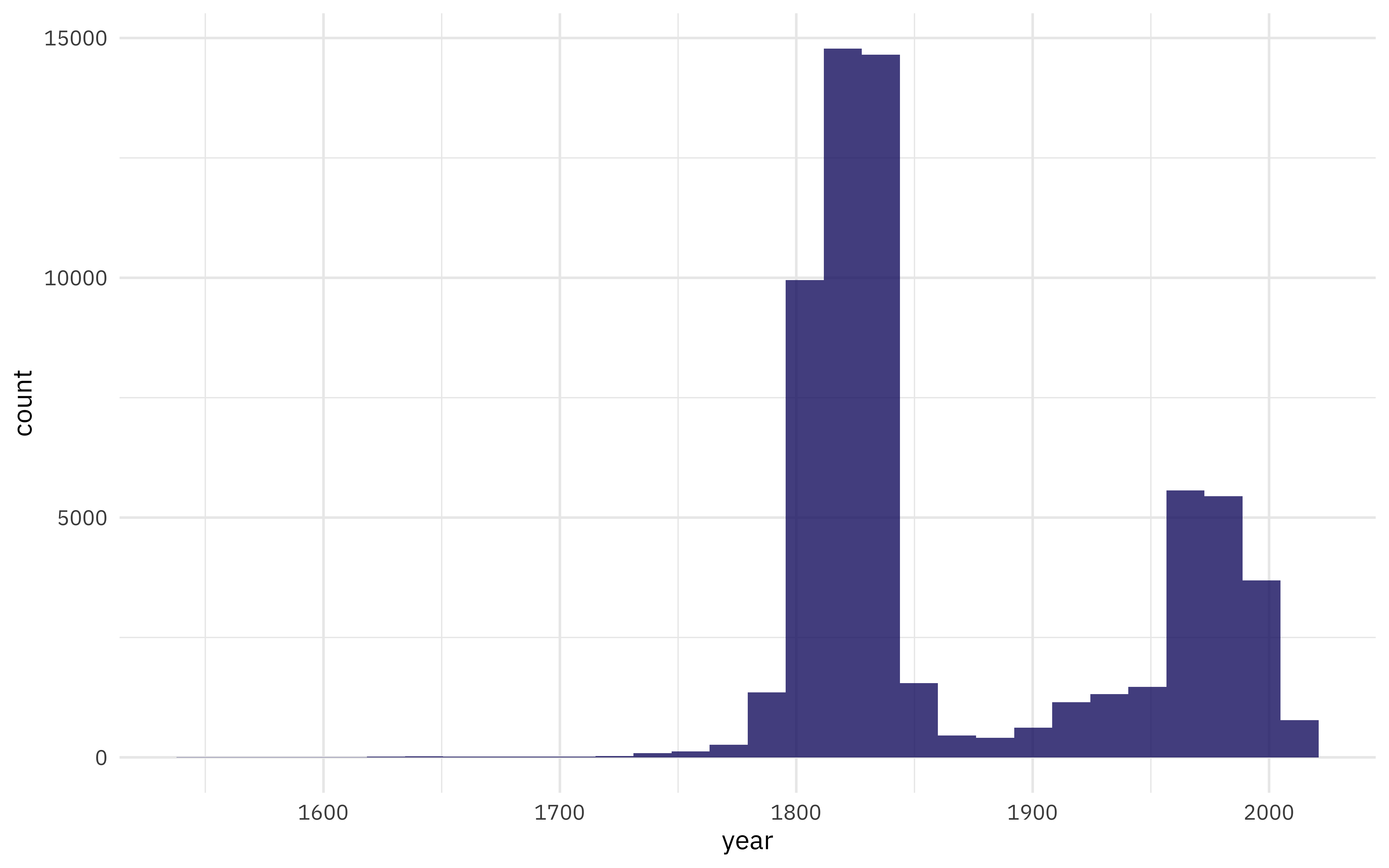
Now this is quite something. I was surprised! I asked on Twitter this week what people thought they would do in a situation where their outcome was distributed like this, and there were lots of interesting thoughts, including “cry”, “ask a lot of questions”, “change careers”. If the goal is to understand how something like medium changes with time, we could dichotomize this variable into something like “new” and “old” art and then train a classification model, or we could just keep this as is and train a regression model, hoping that although the outcome is distributed is a rather odd way, the residuals will turn out OK. (There are lots of other options too, of course.) Let’s walk through how to try this, and how to evaluate the resulting model.

Let’s focus on the variables we’ll use for modeling, and at least focus on just the art created after 1750.

tate_df <- artwork %>%
  filter(year > 1750) %>%
  select(year, medium) %>%
  na.omit() %>%
  arrange(year)

tate_df

## # A tibble: 57,182 x 2
##     year medium
##    <dbl> <chr>
##  1  1751 Oil paint on canvas
##  2  1751 Oil paint on canvas
##  3  1751 Oil paint on canvas
##  4  1751 Etching and engraving on paper
##  5  1751 Oil paint on canvas
##  6  1751 Chalk on paper
##  7  1752 Oil paint on canvas
##  8  1752 Graphite on paper
##  9  1752 Oil paint on canvas
## 10  1752 Etching and engraving on paper
## # … with 57,172 more rows

What are the most common words used in describing the media?

library(tidytext)

tate_df %>%
  unnest_tokens(word, medium) %>%
  count(word, sort = TRUE)

## # A tibble: 1,463 x 2
##    word            n
##    <chr>       <int>
##  1 on          55324
##  2 paper       50134
##  3 graphite    29486
##  4 and         10495
##  5 watercolour  5409
##  6 paint        4961
##  7 oil          4367
##  8 canvas       3644
##  9 screenprint  3422
## 10 lithograph   3015
## # … with 1,453 more rows

Lots of paper, graphite, oil and watercolour paints!

Build a model

We can start by loading the tidymodels metapackage, splitting our data into training and testing sets, and creating resamples.

library(tidymodels)

set.seed(123)
art_split <- initial_split(tate_df, strata = year)
art_train <- training(art_split)
art_test <- testing(art_split)

set.seed(234)
art_folds <- vfold_cv(art_train, strata = year)
art_folds

## #  10-fold cross-validation using stratification
## # A tibble: 10 x 2
##    splits               id
##    <list>               <chr>
##  1 <split [38.6K/4.3K]> Fold01
##  2 <split [38.6K/4.3K]> Fold02
##  3 <split [38.6K/4.3K]> Fold03
##  4 <split [38.6K/4.3K]> Fold04
##  5 <split [38.6K/4.3K]> Fold05
##  6 <split [38.6K/4.3K]> Fold06
##  7 <split [38.6K/4.3K]> Fold07
##  8 <split [38.6K/4.3K]> Fold08
##  9 <split [38.6K/4.3K]> Fold09
## 10 <split [38.6K/4.3K]> Fold10

Next, let’s *preprocess out data to get it ready for modeling. We can use specialized steps from textrecipes, along with the general recipe steps.

library(textrecipes)

art_rec <- recipe(year ~ medium, data = art_train) %>%
  step_tokenize(medium) %>%
  step_stopwords(medium) %>%
  step_tokenfilter(medium, max_tokens = 500) %>%
  step_tfidf(medium)

art_rec

## Data Recipe
##
## Inputs:
##
##       role #variables
##    outcome          1
##  predictor          1
##
## Operations:
##
## Tokenization for medium
## Stop word removal for medium
## Text filtering for medium
## Term frequency-inverse document frequency with medium

Let’s walk through the steps in this recipe, which are what I consider sensible defaults for training a model with text features.

• First, we must tell the recipe() what our model is going to be (using a formula here) and what data we are using.
• Next, we tokenize our text, with the default tokenization into single words.
• Next, we remove stop words (again, just the default set, to remove “on” and “and”).
• It wouldn’t be practical to keep all the tokens from this whole dataset in our model, so we can filter down to only keep, in this case, the top 500 most-used tokens (after removing stop words).
• We need to decide on some kind of weighting for these tokens next, either something like term frequency or, what we used here, tf-idf.

Next, it’s time to specify our model and put it together with our recipe into a workflow. Recently, we added support for sparse data structures to tidymodels, and this is a perfect opportunity to use it for faster model fitting. To use the sparse data structure, create a hardhat blueprint with composition = "dgCMatrix".

sparse_bp <- hardhat::default_recipe_blueprint(composition = "dgCMatrix")

lasso_spec <- linear_reg(penalty = tune(), mixture = 1) %>%
  set_engine("glmnet")

art_wf <- workflow() %>%
  add_recipe(art_rec, blueprint = sparse_bp) %>%
  add_model(lasso_spec)

art_wf

## ══ Workflow ════════════════════════════════════════════════════════════════════
## Preprocessor: Recipe
## Model: linear_reg()
##
## ── Preprocessor ────────────────────────────────────────────────────────────────
## 4 Recipe Steps
##
## ● step_tokenize()
## ● step_stopwords()
## ● step_tokenfilter()
## ● step_tfidf()
##
## ── Model ───────────────────────────────────────────────────────────────────────
## Linear Regression Model Specification (regression)
##
## Main Arguments:
##   penalty = tune()
##   mixture = 1
##
## Computational engine: glmnet

The only other piece we need to get ready for model fitting is values for the regularization penalty to try. The default goes down to very tiny penalties and I don’t think we’ll need that, so let’s change the range().

lambda_grid <- grid_regular(penalty(range = c(-3, 0)), levels = 20)

Now let’s tune the lasso model on the resampled datasets we created.

doParallel::registerDoParallel()
set.seed(1234)

lasso_rs <- tune_grid(
  art_wf,
  resamples = art_folds,
  grid = lambda_grid
)

lasso_rs

## # Tuning results
## # 10-fold cross-validation using stratification
## # A tibble: 10 x 4
##    splits               id     .metrics          .notes
##    <list>               <chr>  <list>            <list>
##  1 <split [38.6K/4.3K]> Fold01 <tibble [40 × 5]> <tibble [0 × 1]>
##  2 <split [38.6K/4.3K]> Fold02 <tibble [40 × 5]> <tibble [0 × 1]>
##  3 <split [38.6K/4.3K]> Fold03 <tibble [40 × 5]> <tibble [0 × 1]>
##  4 <split [38.6K/4.3K]> Fold04 <tibble [40 × 5]> <tibble [0 × 1]>
##  5 <split [38.6K/4.3K]> Fold05 <tibble [40 × 5]> <tibble [0 × 1]>
##  6 <split [38.6K/4.3K]> Fold06 <tibble [40 × 5]> <tibble [0 × 1]>
##  7 <split [38.6K/4.3K]> Fold07 <tibble [40 × 5]> <tibble [0 × 1]>
##  8 <split [38.6K/4.3K]> Fold08 <tibble [40 × 5]> <tibble [0 × 1]>
##  9 <split [38.6K/4.3K]> Fold09 <tibble [40 × 5]> <tibble [0 × 1]>
## 10 <split [38.6K/4.3K]> Fold10 <tibble [40 × 5]> <tibble [0 × 1]>

That was quite fast, because it’s a linear model and we used the sparse data structure.

Evaluate model

Now we can do what we really came here for, which is to talk about how we can evaluate a model like this and see if it was a good idea. How do the results look?

autoplot(lasso_rs)

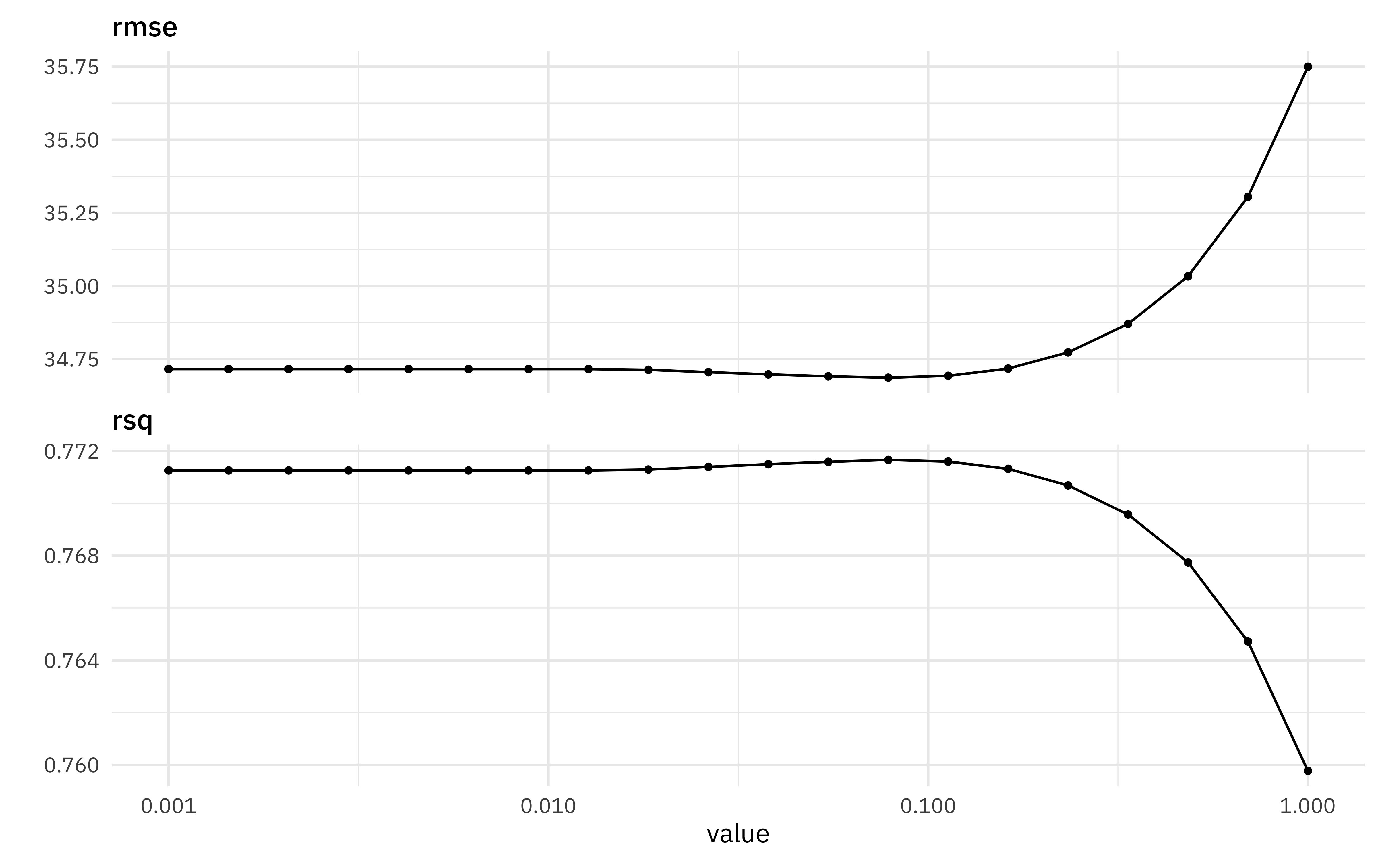
The best $R^2$ is around 0.77, and is a measure of how well the model fits the data. The best RMSE is around 35 or so, and is on the scale of the original outcome, i.e. years. What are some of the best penalty values, in terms of RMSE?

show_best(lasso_rs, "rmse")

## # A tibble: 5 x 7
##   penalty .metric .estimator  mean     n std_err .config
##     <dbl> <chr>   <chr>      <dbl> <int>   <dbl> <chr>
## 1  0.0785 rmse    standard    34.7    10   0.234 Preprocessor1_Model13
## 2  0.0546 rmse    standard    34.7    10   0.235 Preprocessor1_Model12
## 3  0.113  rmse    standard    34.7    10   0.231 Preprocessor1_Model14
## 4  0.0379 rmse    standard    34.7    10   0.237 Preprocessor1_Model11
## 5  0.0264 rmse    standard    34.7    10   0.238 Preprocessor1_Model10

We can select the best penalty, and finalize the workflow with it.

best_rmse <- select_best(lasso_rs, "rmse")

final_lasso <- finalize_workflow(art_wf, best_rmse)
final_lasso

## ══ Workflow ════════════════════════════════════════════════════════════════════
## Preprocessor: Recipe
## Model: linear_reg()
##
## ── Preprocessor ────────────────────────────────────────────────────────────────
## 4 Recipe Steps
##
## ● step_tokenize()
## ● step_stopwords()
## ● step_tokenfilter()
## ● step_tfidf()
##
## ── Model ───────────────────────────────────────────────────────────────────────
## Linear Regression Model Specification (regression)
##
## Main Arguments:
##   penalty = 0.0784759970351461
##   mixture = 1
##
## Computational engine: glmnet

The function last_fit() fits this finalized lasso model one last time to the training data and evaluates one last time on the testing data. The metrics are computed on the testing data.

art_final <- last_fit(final_lasso, art_split)
collect_metrics(art_final)

## # A tibble: 2 x 4
##   .metric .estimator .estimate .config
##   <chr>   <chr>          <dbl> <chr>
## 1 rmse    standard      34.6   Preprocessor1_Model1
## 2 rsq     standard       0.772 Preprocessor1_Model1

We can use the fitted workflow in art_final to explore variable importance using the vip package.

library(vip)

art_vip <- pull_workflow_fit(art_final$.workflow[[1]]) %>%
  vi()


art_vip %>%
  group_by(Sign) %>%
  slice_max(abs(Importance), n = 20) %>%
  ungroup() %>%
  mutate(
    Variable = str_remove(Variable, "tfidf_medium_"),
    Importance = abs(Importance),
    Variable = fct_reorder(Variable, Importance),
    Sign = if_else(Sign == "POS", "More in later art", "More in earlier art")
  ) %>%
  ggplot(aes(Importance, Variable, fill = Sign)) +
  geom_col(show.legend = FALSE) +
  facet_wrap(~Sign, scales = "free") +
  labs(y = NULL)

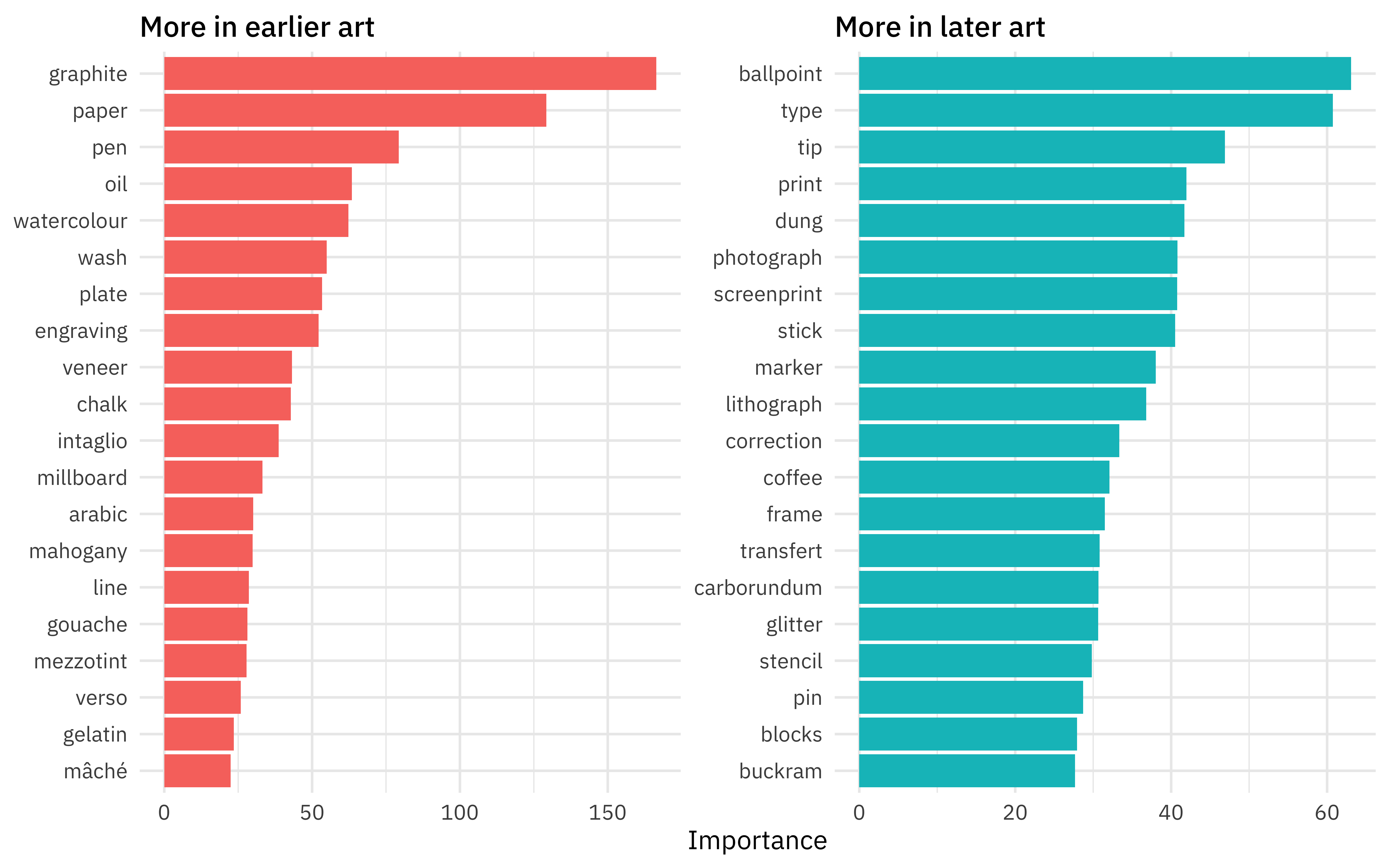
Glitter and dung!!! I am so glad I worked on this model, honestly. This tells quite a story about what predictors are most important in pushing the prediction for an observation up or down the most.

How well does the model actually do, though? Let’s plot true and predicted values for years, for the testing data.

collect_predictions(art_final) %>%
  ggplot(aes(year, .pred)) +
  geom_abline(lty = 2, color = "gray50", size = 1.2) +
  geom_point(size = 1.5, alpha = 0.3, color = "midnightblue") +
  coord_fixed()

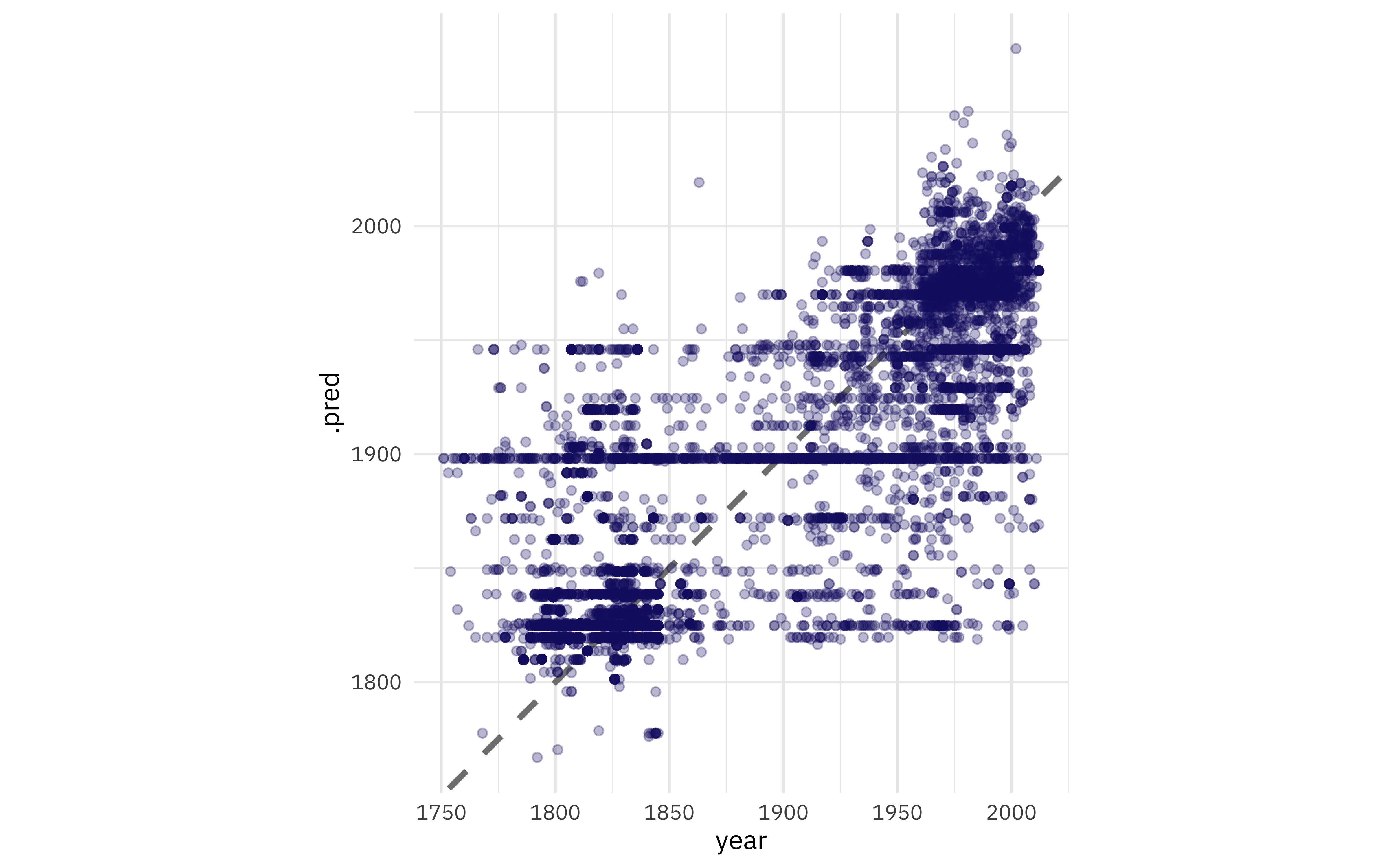
There are clumps of artwork that are predicted well at the high and low end, but notice that prominent horizontal line of observations that are all predicted to be created at about ~1900. Let’s dig more into misclassifications.

misclassified <- collect_predictions(art_final) %>%
  bind_cols(art_test %>% select(medium)) %>%
  filter(abs(year - .pred) > 100)

misclassified %>%
  arrange(year)

## # A tibble: 399 x 6
##    id             .pred  .row  year .config            medium
##    <chr>          <dbl> <int> <dbl> <chr>              <chr>
##  1 train/test sp… 1898.     1  1751 Preprocessor1_Mod… Oil paint on canvas
##  2 train/test sp… 1898.     5  1751 Preprocessor1_Mod… Oil paint on canvas
##  3 train/test sp… 1892.    18  1753 Preprocessor1_Mod… Etching and engraving on…
##  4 train/test sp… 1898.    25  1755 Preprocessor1_Mod… Oil paint on canvas
##  5 train/test sp… 1898.    27  1756 Preprocessor1_Mod… Oil paint on canvas
##  6 train/test sp… 1892.    30  1757 Preprocessor1_Mod… Etching and engraving on…
##  7 train/test sp… 1898.    31  1757 Preprocessor1_Mod… Oil paint on canvas
##  8 train/test sp… 1898.    41  1759 Preprocessor1_Mod… Oil paint on canvas
##  9 train/test sp… 1898.    45  1760 Preprocessor1_Mod… Oil paint on canvas
## 10 train/test sp… 1898.    49  1760 Preprocessor1_Mod… Oil paint on canvas
## # … with 389 more rows

These are pieces of art that were created very early but predicted much later. In fact, notice that “Oil paint on canvas” also predicts to 1898; that is about the mean or median of this whole dataset, that was one of the most common media, and this is how a linear model works!

misclassified %>%
  arrange(-year)

## # A tibble: 399 x 6
##    id            .pred  .row  year .config          medium
##    <chr>         <dbl> <int> <dbl> <chr>            <chr>
##  1 train/test s… 1869. 57179  2012 Preprocessor1_M… Oil paint and graphite on c…
##  2 train/test s… 1898. 57109  2011 Preprocessor1_M… Oil paint on canvas
##  3 train/test s… 1843. 57046  2010 Preprocessor1_M… Mezzotint on paper
##  4 train/test s… 1843. 57049  2010 Preprocessor1_M… Mezzotint on paper
##  5 train/test s… 1868. 57090  2010 Preprocessor1_M… Paper and gouache on paper
##  6 train/test s… 1868. 57094  2010 Preprocessor1_M… Paper and gouache on paper
##  7 train/test s… 1880. 56998  2009 Preprocessor1_M… Oil paint on paper
##  8 train/test s… 1891. 56861  2008 Preprocessor1_M… Etching and graphite on pap…
##  9 train/test s… 1849. 56898  2008 Preprocessor1_M… Ink, watercolour and graphi…
## 10 train/test s… 1880. 56934  2008 Preprocessor1_M… Oil paint on paper
## # … with 389 more rows

These are pieces of art that were created very recently but predicted much earlier. Notice that they have used what we might think of as antique or traditional techniques.

Now, finally, it is time for the residuals. We can compute residuals for the test set with the augment() function.

augment(art_final) %>%
  ggplot(aes(.pred, .resid)) +
  geom_hline(yintercept = 0, lty = 2, color = "gray50", size = 1.2) +
  geom_point(size = 1.5, alpha = 0.3, color = "midnightblue") +
  geom_smooth(color = "black")

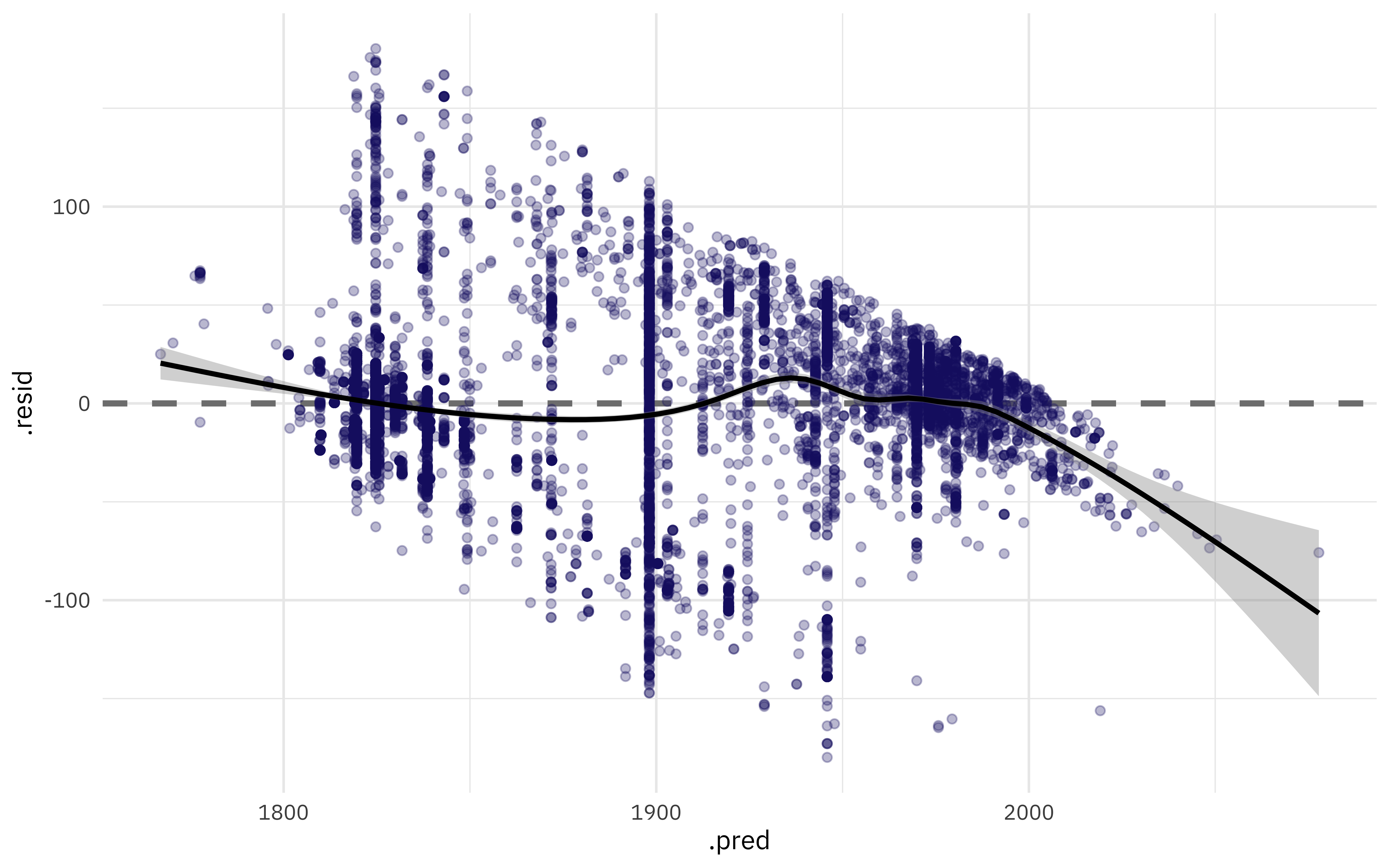
This plot exhibits significant heteroscedasticity, with lower variance for recent artwork and higher variance for older artwork. If the model predicts a recent year, we can be more confident that it is right than if the model predicts an older year, and there is basically no time information in the fact that an artwork was created with a medium like oil on canvas. So is this model bad and not useful? I’d say it’s not great, for most goals I can think of, but it’s interesting to notice how much we can learn about our data even from such a model.