Topic modeling for #TidyTuesday Taylor Swift lyrics
By Julia Silge in rstats
October 23, 2023
This is the latest in my series of
screencasts! I saw Taylor Swift’s Eras Tour movie over the weekend, and this screencast focuses on unsupervised modeling for text with this week’s
#TidyTuesday dataset on the songs of Taylor Swift. Today’s screencast walks through how to build a
structural topic model and then how to understand and interpret it. 💖
Here is the code I used in the video, for those who prefer reading instead of or in addition to video.
Explore data
Our modeling goal is to “discover” topics in the lyrics of Taylor Swift songs. Instead of a supervised or predictive model where our observations have labels, this is an unsupervised approach.
library(tidyverse)
library(taylor)
glimpse(taylor_album_songs)
## Rows: 194
## Columns: 29
## $ album_name          <chr> "Taylor Swift", "Taylor Swift", "Taylor Swift", "T…
## $ ep                  <lgl> FALSE, FALSE, FALSE, FALSE, FALSE, FALSE, FALSE, F…
## $ album_release       <date> 2006-10-24, 2006-10-24, 2006-10-24, 2006-10-24, 2…
## $ track_number        <int> 1, 2, 3, 4, 5, 6, 7, 8, 9, 10, 11, 12, 13, 14, 15,…
## $ track_name          <chr> "Tim McGraw", "Picture To Burn", "Teardrops On My …
## $ artist              <chr> "Taylor Swift", "Taylor Swift", "Taylor Swift", "T…
## $ featuring           <chr> NA, NA, NA, NA, NA, NA, NA, NA, NA, NA, NA, NA, NA…
## $ bonus_track         <lgl> FALSE, FALSE, FALSE, FALSE, FALSE, FALSE, FALSE, F…
## $ promotional_release <date> NA, NA, NA, NA, NA, NA, NA, NA, NA, NA, NA, NA, N…
## $ single_release      <date> 2006-06-19, 2008-02-03, 2007-02-19, NA, NA, NA, N…
## $ track_release       <date> 2006-06-19, 2006-10-24, 2006-10-24, 2006-10-24, 2…
## $ danceability        <dbl> 0.580, 0.658, 0.621, 0.576, 0.418, 0.589, 0.479, 0…
## $ energy              <dbl> 0.491, 0.877, 0.417, 0.777, 0.482, 0.805, 0.578, 0…
## $ key                 <int> 0, 7, 10, 9, 5, 5, 2, 8, 4, 2, 2, 8, 7, 4, 10, 5, …
## $ loudness            <dbl> -6.462, -2.098, -6.941, -2.881, -5.769, -4.055, -4…
## $ mode                <int> 1, 1, 1, 1, 1, 1, 1, 1, 0, 1, 1, 1, 1, 1, 1, 1, 1,…
## $ speechiness         <dbl> 0.0251, 0.0323, 0.0231, 0.0324, 0.0266, 0.0293, 0.…
## $ acousticness        <dbl> 0.57500, 0.17300, 0.28800, 0.05100, 0.21700, 0.004…
## $ instrumentalness    <dbl> 0.00e+00, 0.00e+00, 0.00e+00, 0.00e+00, 0.00e+00, …
## $ liveness            <dbl> 0.1210, 0.0962, 0.1190, 0.3200, 0.1230, 0.2400, 0.…
## $ valence             <dbl> 0.425, 0.821, 0.289, 0.428, 0.261, 0.591, 0.192, 0…
## $ tempo               <dbl> 76.009, 105.586, 99.953, 115.028, 175.558, 112.982…
## $ time_signature      <int> 4, 4, 4, 4, 4, 4, 4, 4, 4, 4, 4, 4, 4, 4, 4, 4, 4,…
## $ duration_ms         <int> 232107, 173067, 203040, 199200, 239013, 207107, 24…
## $ explicit            <lgl> FALSE, FALSE, FALSE, FALSE, FALSE, FALSE, FALSE, F…
## $ key_name            <chr> "C", "G", "A#", "A", "F", "F", "D", "G#", "E", "D"…
## $ mode_name           <chr> "major", "major", "major", "major", "major", "majo…
## $ key_mode            <chr> "C major", "G major", "A# major", "A major", "F ma…
## $ lyrics              <list> [<tbl_df[55 x 4]>], [<tbl_df[33 x 4]>], [<tbl_df[…
Notice that the lyrics variable contains nested tibbles with the texts of the songs; we’ll need to unnest these:
library(tidytext)

tidy_taylor <-
    taylor_album_songs |>
    unnest(lyrics) |>
    unnest_tokens(word, lyric)

tidy_taylor
## # A tibble: 71,721 × 32
##    album_name   ep    album_release track_number track_name artist     featuring
##    <chr>        <lgl> <date>               <int> <chr>      <chr>      <chr>
##  1 Taylor Swift FALSE 2006-10-24               1 Tim McGraw Taylor Sw… <NA>
##  2 Taylor Swift FALSE 2006-10-24               1 Tim McGraw Taylor Sw… <NA>
##  3 Taylor Swift FALSE 2006-10-24               1 Tim McGraw Taylor Sw… <NA>
##  4 Taylor Swift FALSE 2006-10-24               1 Tim McGraw Taylor Sw… <NA>
##  5 Taylor Swift FALSE 2006-10-24               1 Tim McGraw Taylor Sw… <NA>
##  6 Taylor Swift FALSE 2006-10-24               1 Tim McGraw Taylor Sw… <NA>
##  7 Taylor Swift FALSE 2006-10-24               1 Tim McGraw Taylor Sw… <NA>
##  8 Taylor Swift FALSE 2006-10-24               1 Tim McGraw Taylor Sw… <NA>
##  9 Taylor Swift FALSE 2006-10-24               1 Tim McGraw Taylor Sw… <NA>
## 10 Taylor Swift FALSE 2006-10-24               1 Tim McGraw Taylor Sw… <NA>
## # ℹ 71,711 more rows
## # ℹ 25 more variables: bonus_track <lgl>, promotional_release <date>,
## #   single_release <date>, track_release <date>, danceability <dbl>,
## #   energy <dbl>, key <int>, loudness <dbl>, mode <int>, speechiness <dbl>,
## #   acousticness <dbl>, instrumentalness <dbl>, liveness <dbl>, valence <dbl>,
## #   tempo <dbl>, time_signature <int>, duration_ms <int>, explicit <lgl>,
## #   key_name <chr>, mode_name <chr>, key_mode <chr>, line <int>, …
We can find the most common words, or see which words are used the most per song:
tidy_taylor |>
    anti_join(get_stopwords()) |>
    count(track_name, word, sort = TRUE)
## # A tibble: 15,892 × 3
##    track_name                              word      n
##    <chr>                                   <chr> <int>
##  1 Red (Taylor's Version)                  red     107
##  2 I Did Something Bad                     di       81
##  3 Shake It Off                            shake    78
##  4 Wonderland                              eh       72
##  5 Out Of The Woods                        yet      63
##  6 You Need To Calm Down                   oh       63
##  7 I Wish You Would                        wish     62
##  8 State Of Grace (Taylor's Version)       oh       59
##  9 Clean                                   oh       56
## 10 Run (Taylor's Version) [From The Vault] run      52
## # ℹ 15,882 more rows
Train a topic model
To train a topic model with the stm package, we need to create a sparse matrix from our tidy tibble of tokens. Let’s treat each Taylor Swift song as a document, and throw out words used three or fewer times in a song.
lyrics_sparse <-
    tidy_taylor |>
    count(track_name, word) |>
    filter(n > 3) |>
    cast_sparse(track_name, word, n)

dim(lyrics_sparse)
## [1] 194 867
This means there are 191 song (i.e. documents) and different tokens (i.e. terms or words) in our dataset for modeling. Notice that I did not remove stop words here. You typically don’t want to remove stop words before building topic models but we will need to keep in mind that the highest probability words will look mostly the same from each topic.
A topic model like this one models:
- each document as a mixture of topics
- each topic as a mixture of words
The most important parameter when training a topic modeling is K, the number of topics. This is like k in k-means in that it is a hyperparamter of the model and we must choose this value ahead of time. We could
try multiple different values to find the best value for K, but since this is Taylor Swift, let’s use K = 13.
library(stm)
set.seed(123)
topic_model <- stm(lyrics_sparse, K = 13, verbose = FALSE)
To get a quick view of the results, we can use summary().
summary(topic_model)
## A topic model with 13 topics, 194 documents and a 867 word dictionary.

## Topic 1 Top Words:
##  	 Highest Prob: was, you, i, it, the, red, all
##  	 FREX: red, was, there, too, remember, him, well
##  	 Lift: between, hair, prayer, rare, sacred, stairs, wind
##  	 Score: red, there, him, was, well, too, remember
## Topic 2 Top Words:
##  	 Highest Prob: you, and, the, i, a, me, to
##  	 FREX: smile, not, jump, she, everybody, belong, la
##  	 Lift: road, taken, told, okay, ours, single, vow
##  	 Score: la, knows, she, smile, she's, jump, times
## Topic 3 Top Words:
##  	 Highest Prob: i, the, you, and, know, me, my
##  	 FREX: daylight, trouble, know, bye, places, street, cornelia
##  	 Lift: lose, anything, daylight, shoulda, flew, places, shame
##  	 Score: places, daylight, trouble, he's, bye, street, cornelia
## Topic 4 Top Words:
##  	 Highest Prob: the, we, in, and, of, a, are
##  	 FREX: woods, clear, car, getaway, starlight, run, are
##  	 Lift: ridin, bring, pretenders, screaming, careful, careless, daughter
##  	 Score: clear, yet, woods, run, are, out, starlight
## Topic 5 Top Words:
##  	 Highest Prob: oh, you, this, the, and, is, to
##  	 FREX: oh, asking, grow, this, last, twenty, fallin
##  	 Lift: goin, how'd, plane, top, anymore, alright, promises
##  	 Score: oh, last, asking, grow, love, come, fallin
## Topic 6 Top Words:
##  	 Highest Prob: a, you, the, i, and, it, if
##  	 FREX: beautiful, karma, blood, we've, man, if, fairytale
##  	 Lift: blood, cut, we've, boyfriend, fast, ruining, deep
##  	 Score: man, we've, blood, karma, beautiful, fairytale, today
## Topic 7 Top Words:
##  	 Highest Prob: ooh, the, you, i, and, ah, to
##  	 FREX: ooh, ah, once, talk, e, whoa, ever
##  	 Lift: count, keeping, cruel, roll, high, infidelity, woo
##  	 Score: ooh, ah, dorothea, once, you'll, e, whoa
## Topic 8 Top Words:
##  	 Highest Prob: di, eh, i, you, and, it, so
##  	 FREX: di, eh, da, wonderland, over, didn't, good
##  	 Lift: felt, wonderland, alive, dead, died, da, eh
##  	 Score: di, eh, da, wonderland, over, why's, alive
## Topic 9 Top Words:
##  	 Highest Prob: you, to, the, it's, i, me, but
##  	 FREX: york, welcome, mr, snow, beach, new, i've
##  	 Lift: flying, both, quite, beat, bright, agrees, hi
##  	 Score: york, welcome, new, mr, snow, beach, hold
## Topic 10 Top Words:
##  	 Highest Prob: you, i, and, the, be, don't, to
##  	 FREX: bet, big, wish, would, come, help, wanna
##  	 Lift: guiding, spend, wonderstruck, stephen, slope, learned, read
##  	 Score: wish, bet, come, wanna, would, mean, big
## Topic 11 Top Words:
##  	 Highest Prob: i, it, you, what, me, the, want
##  	 FREX: shake, isn't, fake, want, call, off, gorgeous
##  	 Lift: turns, caught, crime, lettin, until, baby's, isn't
##  	 Score: shake, isn't, off, fake, call, look, hate
## Topic 12 Top Words:
##  	 Highest Prob: and, i, when, you, the, oh, it
##  	 FREX: when, rains, that's, girl, said, back, finally
##  	 Lift: shimmer, after, behind, realized, bejeweled, polish, any
##  	 Score: when, rains, finally, that's, clean, oh, works
## Topic 13 Top Words:
##  	 Highest Prob: my, you, the, i, me, to, in
##  	 FREX: my, left, take, ha, usin, rest, bought
##  	 Lift: lovin, betty, party, showed, goddamn, house, stone
##  	 Score: ha, other, take, left, usin, cuts, thousand
Notice that we do in fact have fairly uninteresting and common words as the most common for all the topics. This is because we did not remove stopwords.
Explore topic model results
To explore more deeply, we can tidy() the topic model results to get a dataframe that we can compute on. If we did tidy(topic_model) that would give us the matrix of topic-word probabilities, i.e. the highest probability words from each topic. This is the boring one that is mostly common words like “you” and “me”.
We can alternatively use other metrics for identifying important words, like FREX (high frequency and high exclusivity) or lift:
tidy(topic_model, matrix = "lift")
## # A tibble: 11,271 × 2
##    topic term
##    <int> <chr>
##  1     1 between
##  2     1 hair
##  3     1 prayer
##  4     1 rare
##  5     1 sacred
##  6     1 stairs
##  7     1 wind
##  8     1 lock
##  9     1 palm
## 10     1 why'd
## # ℹ 11,261 more rows
This returns a ranked set of words (not the underlying metrics themselves) and gives us a much clearer idea of what makes each topic unique! Topic 1 looks to be more from the Red album.
We also can use tidy() to get the matrix of document-topic probabilities. For this, we need to pass in the document_names:
lyrics_gamma <- tidy(
  topic_model,
  matrix = "gamma",
  document_names = rownames(lyrics_sparse)
)
How are these topics related to Taylor Swift’s eras (i.e. albums)?
lyrics_gamma |>
    left_join(
        taylor_album_songs |>
            select(album_name, document = track_name) |>
            mutate(album_name = fct_inorder(album_name))
    ) |>
    mutate(topic = factor(topic)) |>
    ggplot(aes(gamma, topic, fill = topic)) +
    geom_boxplot(alpha = 0.7, show.legend = FALSE) +
    facet_wrap(vars(album_name)) +
    labs(x = expression(gamma))
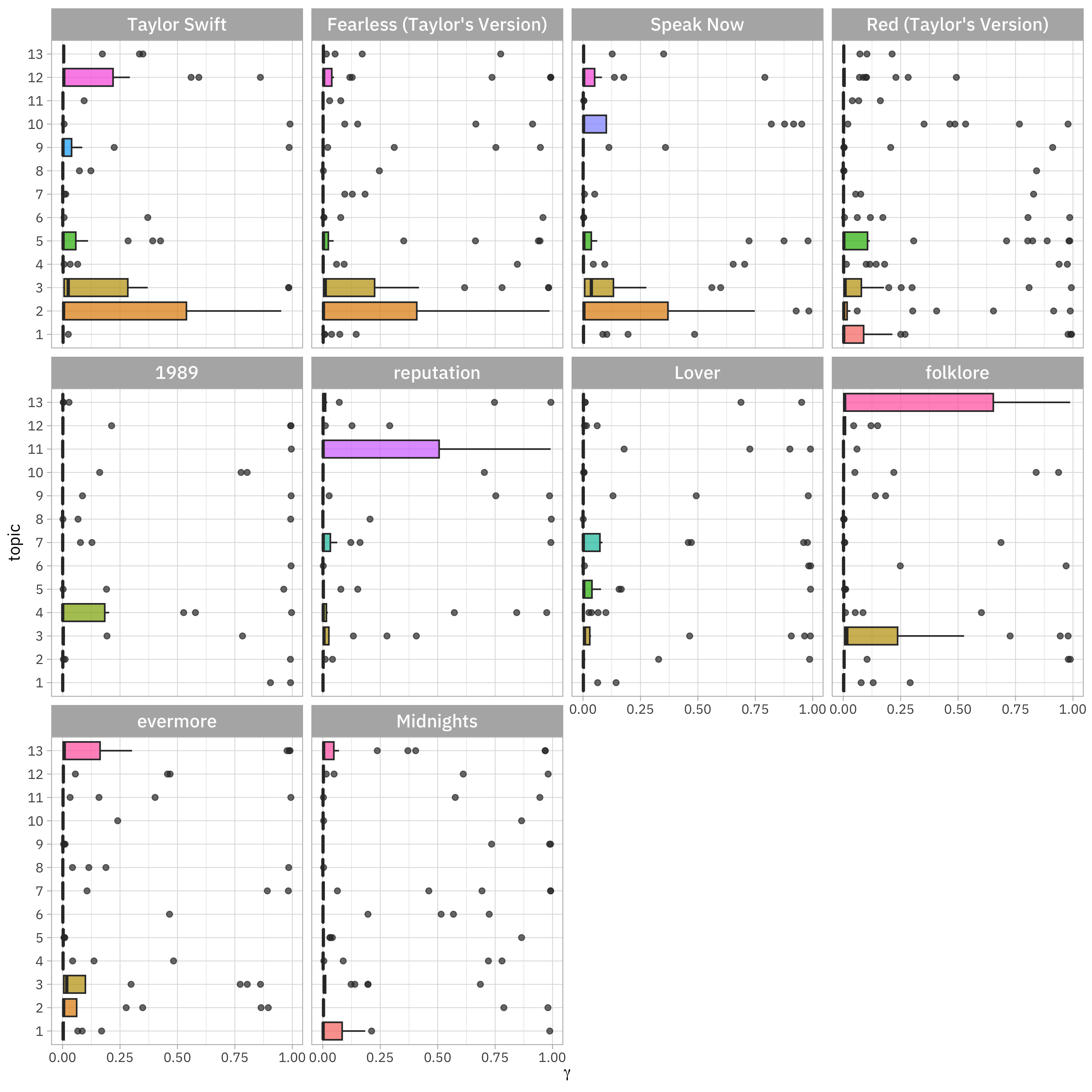
Topics 2 and 3 look to be more prevalent in Taylor Swift’s early albums, Topic 1 does look to be mostly from Red, and topic 13 is uncommon except in folklore and evermore.
Estimate topic effects
There is a TON more you can do with topic models. For example, we can take the trained topic model and, using some supplementary metadata on our documents, estimate regressions for the proportion of each document about a topic with the metadata as the predictors. For example, let’s estimate regressions for our topics with the album name as the predictor. This asks the statistical question, “Do the topics in Taylor Swift songs change across albums?” We looked at this question visually in the last section, but now we can build a model to look at it a different way.
set.seed(123)

effects <-
  estimateEffect(
    1:13 ~ album_name,
    topic_model,
    taylor_album_songs |> distinct(track_name, album_name) |> arrange(track_name)
  )
You can use summary(effects) to see some results here, but you also can tidy() the output to be able to compute on it. Do we have evidence for any of the topics being related to album, in the sense of having a p-value less than 0.05?
tidy(effects) |>
    filter(term != "(Intercept)", p.value < 0.05)
## # A tibble: 3 × 6
##   topic term                 estimate std.error statistic p.value
##   <int> <chr>                   <dbl>     <dbl>     <dbl>   <dbl>
## 1    11 album_namereputation    0.175    0.0815      2.15 0.0329
## 2    13 album_nameevermore      0.184    0.0926      1.99 0.0479
## 3    13 album_namefolklore      0.245    0.0906      2.71 0.00745
Here we see evidence that there is more topic 11 from reputation and more topic 13 in both folklore and evermore. Certainly they are lyrically pretty distinct from her other work! What are some of the highest lift words for this topic?
tidy(topic_model, matrix = "lift") |>
  filter(topic == 13)
## # A tibble: 867 × 2
##    topic term
##    <int> <chr>
##  1    13 lovin
##  2    13 betty
##  3    13 party
##  4    13 showed
##  5    13 goddamn
##  6    13 house
##  7    13 stone
##  8    13 peace
##  9    13 cuts
## 10    13 death
## # ℹ 857 more rows