Training, evaluating, and interpreting topic models

Modeling the Hacker News corpus

In my last blog post, I demonstrated how to get started with about a book’s worth of text, which is a TEENY TINY amount of text for a topic model. This time around, I’d like to demonstrate how to go about interpreting results with a more realistic set of text, something more like what you might actually want to model topics with in the real world, so let’s turn to the Hacker news corpus and download 100,000 texts using the bigrquery package.

library(bigrquery)
library(tidyverse)

sql <- "#legacySQL
SELECT
  stories.title AS title,
  stories.text AS text,
FROM
  [bigquery-public-data:hacker_news.full] AS stories
WHERE
  stories.deleted IS NULL
LIMIT
  100000"

hacker_news_raw <- query_exec(sql, project = project, max_pages = Inf)

After we have the text downloaded, let’s clean the text and make a data frame containing only the text, plus an ID to identify each “document”, i.e., post.

hacker_news_text <- hacker_news_raw %>%
  as_tibble() %>%
  mutate(title = na_if(title, ""),
         text = coalesce(title, text)) %>%
  select(-title) %>%
  mutate(text = str_replace_all(text, "&#x27;|&quot;|&#x2F;", "'"), ## weird encoding
         text = str_replace_all(text, "<a(.*?)>", " "),             ## links 
         text = str_replace_all(text, "&gt;|&lt;|&amp;", " "),      ## html yuck
         text = str_replace_all(text, "&#[:digit:]+;", " "),        ## html yuck
         text = str_remove_all(text, "<[^>]*>"),                    ## mmmmm, more html yuck
         postID = row_number()) 

Now it’s time to tokenize and tidy the text, remove some stop words (and numbers, although this is an analytical choice that you might want to try in a different way), and then cast to a sparse matrix. I’m using the token = "tweets" option for tokenizing because it often performs the most sensibly with text from online forums, such as Hacker News (and Stack Overflow, and Reddit, and so on). In my previous blog post, I used a quanteda dfm as the input to the topic modeling algorithm, but here I’m using a plain old sparse matrix. Either one works.

library(tidytext)

tidy_hacker_news <- hacker_news_text %>%
  unnest_tokens(word, text, token = "tweets") %>%
  anti_join(get_stopwords()) %>%
  filter(!str_detect(word, "[0-9]+")) %>%
  add_count(word) %>%
  filter(n > 100) %>%
  select(-n)

hacker_news_sparse <- tidy_hacker_news %>%
  count(postID, word) %>%
  cast_sparse(postID, word, n)

Train and evaluate topic models

Now it’s time to train some topic models! 💪 You can check out that previous blog post on stm for some details on how to get started, but in this post, we’re going to go to the next level. We’re not going to train just one topic model, but a whole group of them, with different numbers of topics, and then evaluate these models. In topic modeling, like with k-means clustering, we don’t know ahead of time how many topics we should use, and research in this area says there is no “right” answer for the number of topics that is appropriate for any given corpus. Here, let’s try a number of different values for \(K\) (the number of topics) from 20 to 100.

With 100,000 texts this modeling takes a while 😩 so I have used I have used the furrr package (and future) for parallel processing.

library(stm)
library(furrr)
plan(multiprocess)

many_models <- data_frame(K = c(20, 40, 50, 60, 70, 80, 100)) %>%
  mutate(topic_model = future_map(K, ~stm(hacker_news_sparse, K = .,
                                          verbose = FALSE)))

Now that we’ve fit all these topic models with different numbers of topics, we can explore how many topics are appropriate/good/“best”. The code below to find k_result is similar to stm’s own searchK() function, but it allows you to evaluate models trained on a sparse matrix (or a quanteda dfm) instead of only stm’s corpus data structure, as well as to dig into the model diagnostics yourself in detail. Some of these functions were not originally flexible enough to take a sparse matrix or dfm as input, so I’d like to send huge thanks to Brandon Stewart, stm’s developer, for adding this functionality.

heldout <- make.heldout(hacker_news_sparse)

k_result <- many_models %>%
  mutate(exclusivity = map(topic_model, exclusivity),
         semantic_coherence = map(topic_model, semanticCoherence, hacker_news_sparse),
         eval_heldout = map(topic_model, eval.heldout, heldout$missing),
         residual = map(topic_model, checkResiduals, hacker_news_sparse),
         bound =  map_dbl(topic_model, function(x) max(x$convergence$bound)),
         lfact = map_dbl(topic_model, function(x) lfactorial(x$settings$dim$K)),
         lbound = bound + lfact,
         iterations = map_dbl(topic_model, function(x) length(x$convergence$bound)))

k_result

## # A tibble: 7 x 10
##       K topic_model exclusivity semantic_coherence eval_heldout residual        bound lfact     lbound iterations
##   <dbl> <list>      <list>      <list>             <list>       <list>          <dbl> <dbl>      <dbl>      <dbl>
## 1    20 <S3: STM>   <dbl [20]>  <dbl [20]>         <list [4]>   <list [3]> -15991207.  42.3 -15991165.         19
## 2    40 <S3: STM>   <dbl [40]>  <dbl [40]>         <list [4]>   <list [3]> -15990161. 110.  -15990051.         26
## 3    50 <S3: STM>   <dbl [50]>  <dbl [50]>         <list [4]>   <list [3]> -15998161. 148.  -15998012.         30
## 4    60 <S3: STM>   <dbl [60]>  <dbl [60]>         <list [4]>   <list [3]> -16014305. 189.  -16014117.         33
## 5    70 <S3: STM>   <dbl [70]>  <dbl [70]>         <list [4]>   <list [3]> -16007921. 230.  -16007690.         41
## 6    80 <S3: STM>   <dbl [80]>  <dbl [80]>         <list [4]>   <list [3]> -16018471. 274.  -16018197.         48
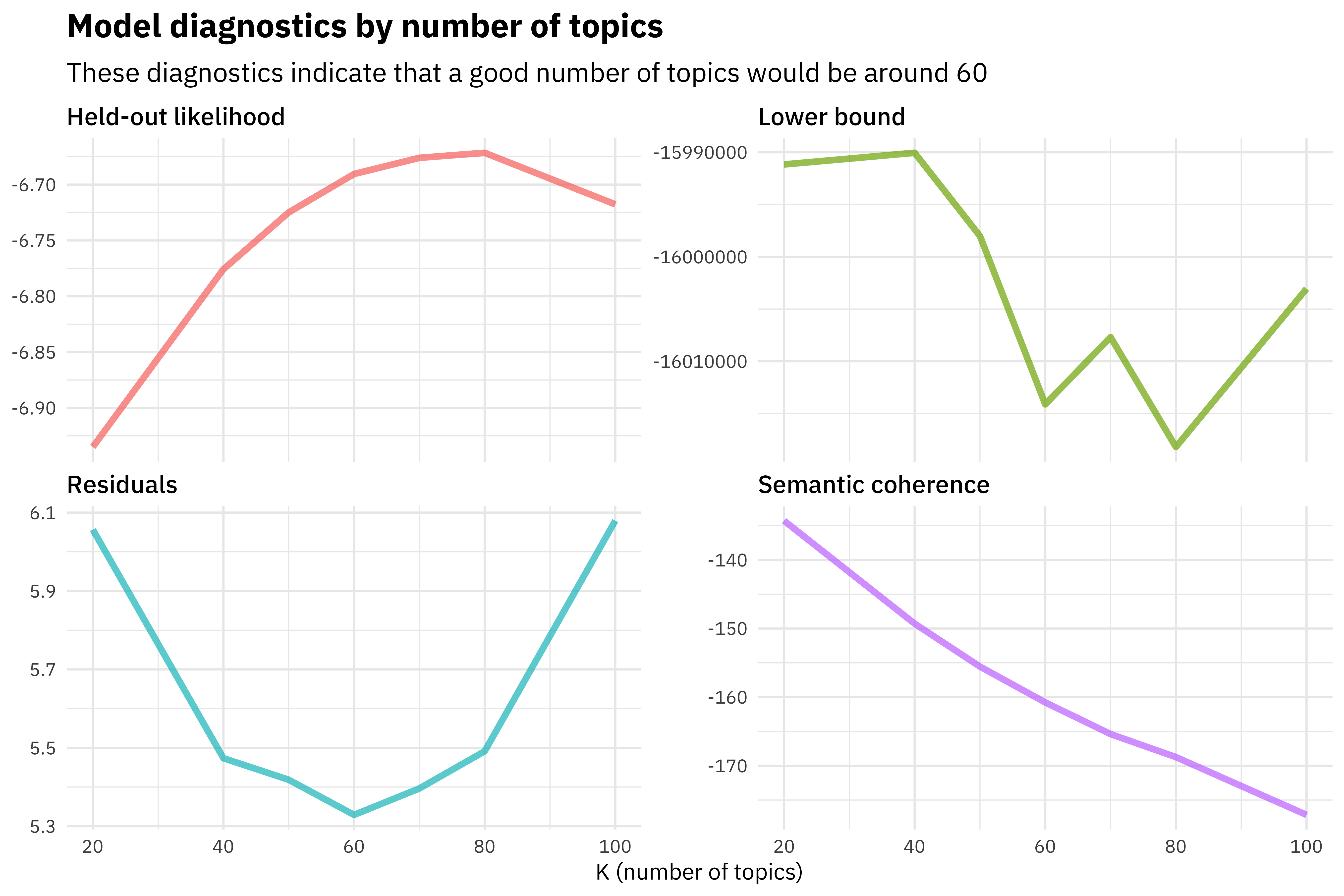
## 7   100 <S3: STM>   <dbl [100]> <dbl [100]>        <list [4]>   <list [3]> -16003418. 364.  -16003055.        114

We’re evaluating things like the residuals, the semantic coherence of the topics, the likelihood for held-out datasets, and more. We can make some diagnostic plots using these quantities to understand how the models are performing at various numbers of topics. The following code makes a diagnostic plot similar to one that comes built in to the stm package.

k_result %>%
  transmute(K,
            `Lower bound` = lbound,
            Residuals = map_dbl(residual, "dispersion"),
            `Semantic coherence` = map_dbl(semantic_coherence, mean),
            `Held-out likelihood` = map_dbl(eval_heldout, "expected.heldout")) %>%
  gather(Metric, Value, -K) %>%
  ggplot(aes(K, Value, color = Metric)) +
  geom_line(size = 1.5, alpha = 0.7, show.legend = FALSE) +
  facet_wrap(~Metric, scales = "free_y") +
  labs(x = "K (number of topics)",
       y = NULL,
       title = "Model diagnostics by number of topics",
       subtitle = "These diagnostics indicate that a good number of topics would be around 60")

The held-out likelihood is highest between 60 and 80, and the residuals are lowest around 60, so perhaps a good number of topics would be around there.

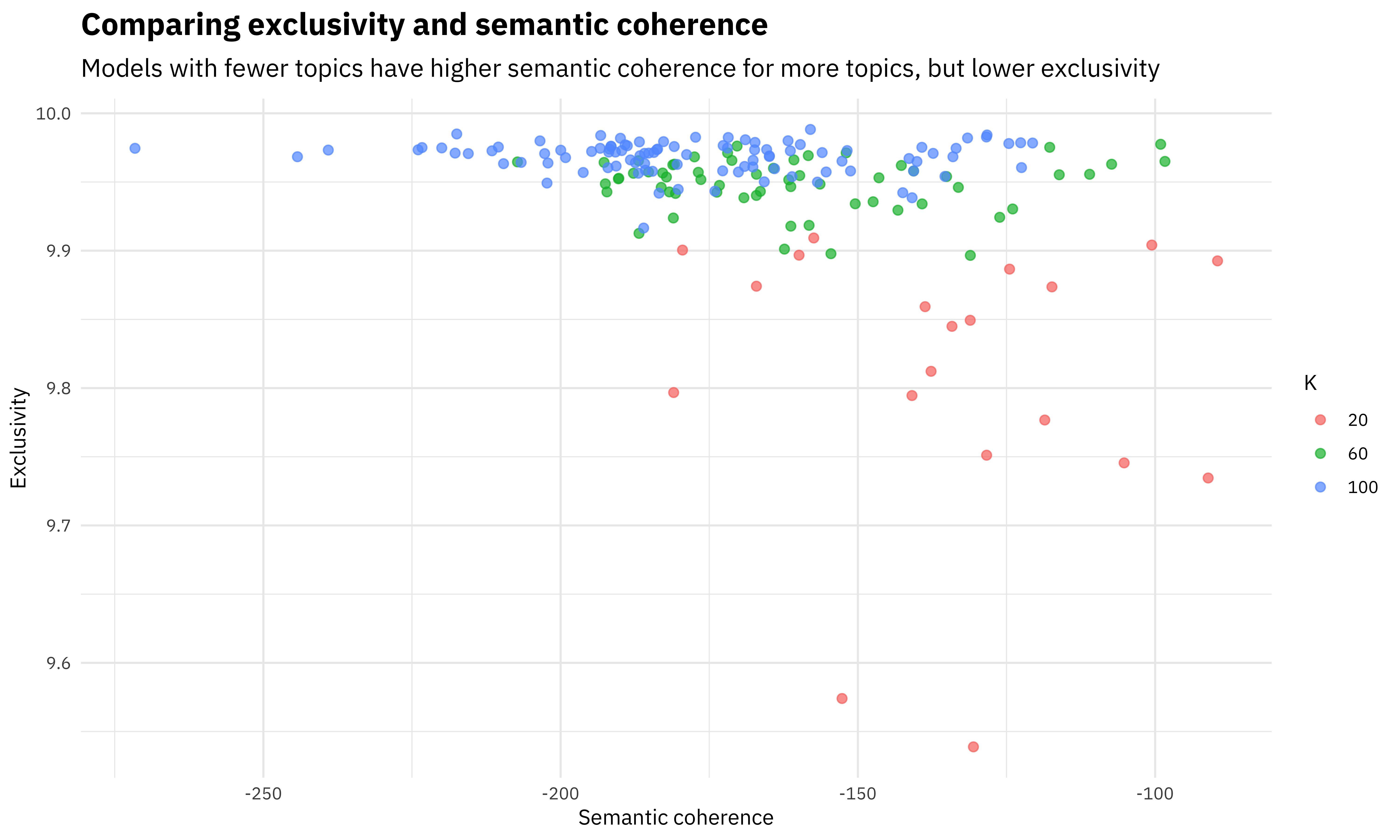
Semantic coherence is maximized when the most probable words in a given topic frequently co-occur together, and it’s a metric that correlates well with human judgment of topic quality. Having high semantic coherence is relatively easy, though, if you only have a few topics dominated by very common words, so you want to look at both semantic coherence and exclusivity of words to topics. It’s a tradeoff. Read more about semantic coherence in the original paper about it.

k_result %>%
  select(K, exclusivity, semantic_coherence) %>%
  filter(K %in% c(20, 60, 100)) %>%
  unnest() %>%
  mutate(K = as.factor(K)) %>%
  ggplot(aes(semantic_coherence, exclusivity, color = K)) +
  geom_point(size = 2, alpha = 0.7) +
  labs(x = "Semantic coherence",
       y = "Exclusivity",
       title = "Comparing exclusivity and semantic coherence",
       subtitle = "Models with fewer topics have higher semantic coherence for more topics, but lower exclusivity")

So for this analysis, it looks a good choice could be the model with 60 topics.

topic_model <- k_result %>% 
  filter(K == 60) %>% 
  pull(topic_model) %>% 
  .[[1]]

topic_model

## A topic model with 60 topics, 98000 documents and a 3828 word dictionary.

Explore the topic model

We’ve trained topic models, evaluated them, and picked one to use, so now let’s see what this topic model tells us about the Hacker News corpus. In real life analysis, this process would be iterative, moving from exploring and interpreting a model back and forth to diagnostics and evaluation in order to decide how best to model a corpus. One of the reasons I embrace tidy data principles and tidy tools is that this iterative process is streamlined. For example, let’s tidy() the beta matrix for our topic model and look at the probabilities that each word is generated from each topic.

td_beta <- tidy(topic_model)

td_beta

## # A tibble: 229,680 x 3
##    topic term          beta
##    <int> <chr>        <dbl>
##  1     1 arguments 8.56e-20
##  2     2 arguments 4.20e-15
##  3     3 arguments 3.21e-15
##  4     4 arguments 9.23e-13
##  5     5 arguments 1.45e-12
##  6     6 arguments 5.44e-18
##  7     7 arguments 1.04e-24
##  8     8 arguments 1.52e-11
##  9     9 arguments 4.77e-16
## 10    10 arguments 2.29e-16
## # ... with 229,670 more rows

I’m also quite interested in the probabilities that each document is generated from each topic, that gamma matrix.

td_gamma <- tidy(topic_model, matrix = "gamma",
                 document_names = rownames(hacker_news_sparse))

td_gamma

## # A tibble: 5,880,000 x 3
##    document topic   gamma
##    <chr>    <int>   <dbl>
##  1 1            1 0.00631
##  2 2            1 0.00446
##  3 3            1 0.00670
##  4 4            1 0.00767
##  5 5            1 0.00742
##  6 6            1 0.00907
##  7 7            1 0.00479
##  8 8            1 0.00906
##  9 9            1 0.00801
## 10 10           1 0.00881
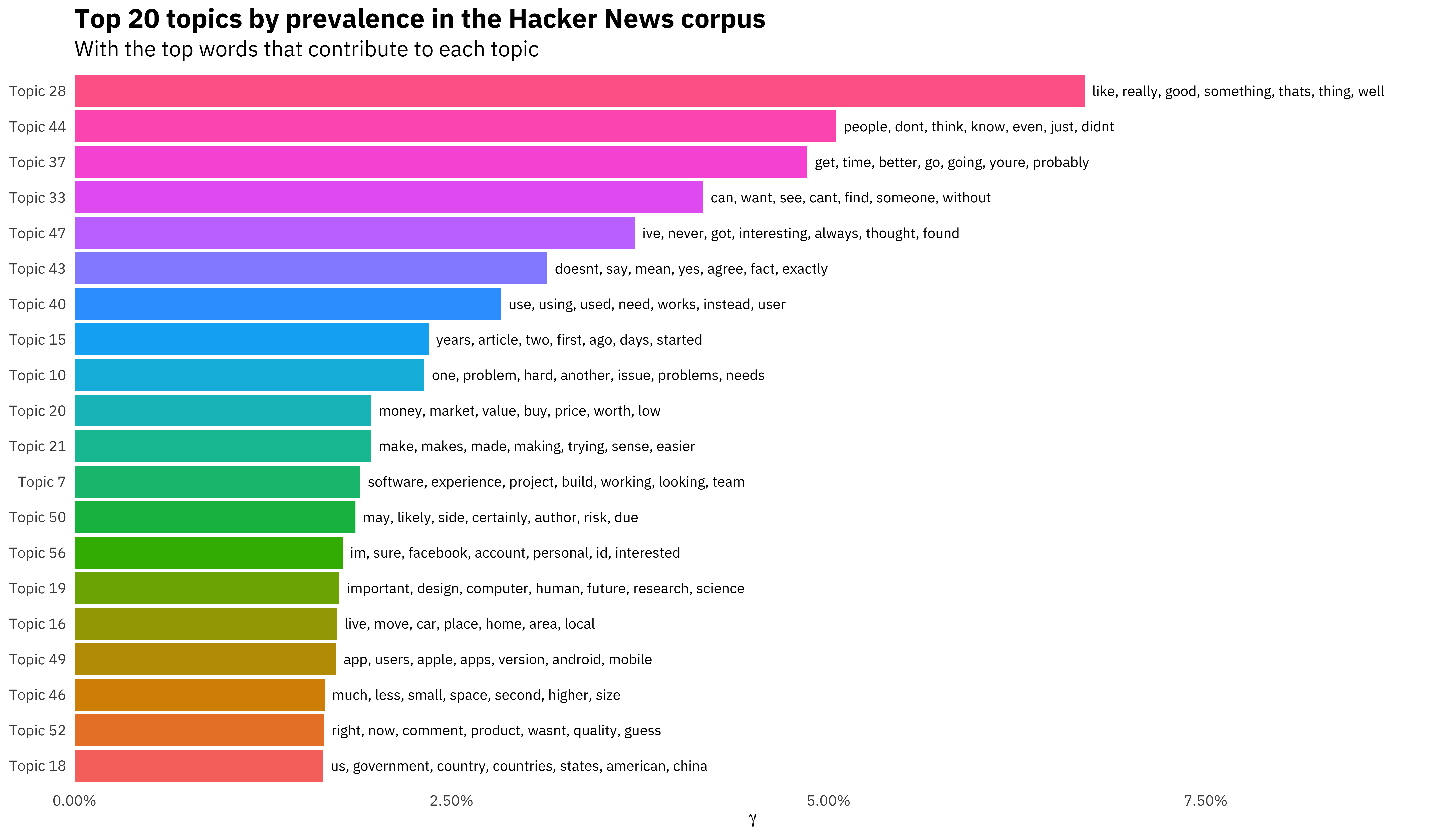
## # ... with 5,879,990 more rows

Let’s combine these to understand the topic prevalence in the Hacker News corpus, and which words contribute to each topic.

library(ggthemes)

top_terms <- td_beta %>%
  arrange(beta) %>%
  group_by(topic) %>%
  top_n(7, beta) %>%
  arrange(-beta) %>%
  select(topic, term) %>%
  summarise(terms = list(term)) %>%
  mutate(terms = map(terms, paste, collapse = ", ")) %>% 
  unnest()

gamma_terms <- td_gamma %>%
  group_by(topic) %>%
  summarise(gamma = mean(gamma)) %>%
  arrange(desc(gamma)) %>%
  left_join(top_terms, by = "topic") %>%
  mutate(topic = paste0("Topic ", topic),
         topic = reorder(topic, gamma))

gamma_terms %>%
  top_n(20, gamma) %>%
  ggplot(aes(topic, gamma, label = terms, fill = topic)) +
  geom_col(show.legend = FALSE) +
  geom_text(hjust = 0, nudge_y = 0.0005, size = 3,
            family = "IBMPlexSans") +
  coord_flip() +
  scale_y_continuous(expand = c(0,0),
                     limits = c(0, 0.09),
                     labels = percent_format()) +
  theme_tufte(base_family = "IBMPlexSans", ticks = FALSE) +
  theme(plot.title = element_text(size = 16,
                                  family="IBMPlexSans-Bold"),
        plot.subtitle = element_text(size = 13)) +
  labs(x = NULL, y = expression(gamma),
       title = "Top 20 topics by prevalence in the Hacker News corpus",
       subtitle = "With the top words that contribute to each topic")

We can look at all the topics, ordered by prevalence.

gamma_terms %>%
  select(topic, gamma, terms) %>%
  kable(digits = 3, 
        col.names = c("Topic", "Expected topic proportion", "Top 7 terms"))

Topic	Expected topic proportion	Top 7 terms
Topic 28	0.067	like, really, good, something, thats, thing, well
Topic 44	0.050	people, dont, think, know, even, just, didnt
Topic 37	0.049	get, time, better, go, going, youre, probably
Topic 33	0.042	can, want, see, cant, find, someone, without
Topic 47	0.037	ive, never, got, interesting, always, thought, found
Topic 43	0.031	doesnt, say, mean, yes, agree, fact, exactly
Topic 40	0.028	use, using, used, need, works, instead, user
Topic 15	0.023	years, article, two, first, ago, days, started
Topic 10	0.023	one, problem, hard, another, issue, problems, needs
Topic 20	0.020	money, market, value, buy, price, worth, low
Topic 21	0.020	make, makes, made, making, trying, sense, easier
Topic 7	0.019	software, experience, project, build, working, looking, team
Topic 50	0.019	may, likely, side, certainly, author, risk, due
Topic 56	0.018	im, sure, facebook, account, personal, id, interested
Topic 19	0.018	important, design, computer, human, future, research, science
Topic 16	0.017	live, move, car, place, home, area, local
Topic 49	0.017	app, users, apple, apps, version, android, mobile
Topic 46	0.017	much, less, small, space, second, higher, size
Topic 52	0.017	right, now, comment, product, wasnt, quality, guess
Topic 18	0.016	us, government, country, countries, states, american, china
Topic 51	0.016	year, support, last, old, next, linux, per
Topic 17	0.015	language, programming, c, learn, python, languages, written
Topic 12	0.014	company, business, startup, name, ideas, early, employees
Topic 2	0.014	part, real, reason, life, story, guy, bitcoin
Topic 31	0.014	code, open, source, write, writing, test, program
Topic 22	0.014	pay, cost, paid, costs, paying, rate, amount
Topic 9	0.013	email, ask, show, best, link, please, form
Topic 54	0.013	system, large, control, systems, built, scale, require
Topic 55	0.013	wrong, nothing, page, difference, whats, theres, view
Topic 26	0.013	case, law, cases, nobody, wants, serious, laws
Topic 53	0.013	change, group, history, position, political, involved, individual
Topic 25	0.012	read, top, list, reading, add, news, books
Topic 11	0.012	google, internet, search, browser, ie, address, chrome
Topic 39	0.012	standard, eg, types, implementation, object, structure, table
Topic 42	0.012	new, create, technology, website, rules, existing, created
Topic 38	0.012	high, school, tax, average, poor, course, kids
Topic 30	0.012	run, running, server, api, application, client, database
Topic 35	0.012	data, information, public, access, private, analysis, details
Topic 48	0.012	line, available, video, tools, vs, basic, tool
Topic 24	0.012	different, true, model, definitely, yeah, left, completely
Topic 41	0.011	service, services, provide, customers, called, trust, customer
Topic 36	0.011	game, play, games, fun, sound, water, playing
Topic 34	0.011	almost, fast, extremely, field, speed, tend, theory
Topic 5	0.011	person, must, common, wonder, situation, along, net
Topic 29	0.011	example, type, call, result, function, lack, currently
Topic 59	0.011	number, phone, =, +, numbers, normal, random
Topic 60	0.011	also, just, still, already, well, way, least
Topic 14	0.011	free, windows, full, online, key, microsoft, offer
Topic 3	0.011	work, job, state, book, jobs, leave, hire
Topic 27	0.010	world, security, talking, rest, parts, seeing, changed
Topic 13	0.010	web, site, post, x, os, sites, blog
Topic 23	0.010	power, become, benefit, society, food, energy, cars
Topic 32	0.009	often, sometimes, word, ones, words, turn, context
Topic 1	0.009	question, level, whether, answer, questions, asked, asking
Topic 57	0.009	set, simple, default, complex, relatively, push, implement
Topic 6	0.009	big, companies, many, tech, deal, industry, huge
Topic 45	0.008	content, social, network, results, media, ads, ad
Topic 8	0.008	file, terms, legal, files, step, purpose, license
Topic 4	0.008	women, culture, age, men, young, people, older
Topic 58	0.006	hn, community, light, others, reddit, come, hey

We can see here that the first several topics are focused around general purpose English words in different categories of meaning. About 10 topics down, we see a topic about markets, money, and value. A bit below that, we see the first topic with explicitly technical-ish terms like software, build, and project. There is a topic that combined “make”, “makes”, “made”, and “making”. Notice that I did not stem these words before modeling. Research shows that stemming words when topic modeling doesn’t help and often hurts, so don’t automatically assume that you should be stemming your words.

So there you have it! We trained topic models at multiple values of \(K\), evaluated them, and then explored our model. Let me know if you have any questions or feedback!