Bagging with tidymodels and #TidyTuesday astronaut missions

Lately I’ve been publishing screencasts demonstrating how to use the tidymodels framework, from first steps in modeling to how to evaluate complex models. Today’s screencast focuses on bagging using this week’s #TidyTuesday dataset on astronaut missions. 👩‍🚀

Here is the code I used in the video, for those who prefer reading instead of or in addition to video.

Explore the data

Our modeling goal is to use bagging (bootstrap aggregation) to model the duration of astronaut missions from this week’s #TidyTuesday dataset.

Let’s start by reading in the data and check out what the top spacecraft used in orbit have been.

astronauts <- read_csv("https://raw.githubusercontent.com/rfordatascience/tidytuesday/master/data/2020/2020-07-14/astronauts.csv")

astronauts %>%
  count(in_orbit, sort = TRUE)

## # A tibble: 289 x 2
##    in_orbit      n
##    <chr>     <int>
##  1 ISS         174
##  2 Mir          71
##  3 Salyut 6     24
##  4 Salyut 7     24
##  5 STS-42        8
##  6 explosion     7
##  7 STS-103       7
##  8 STS-107       7
##  9 STS-109       7
## 10 STS-110       7
## # … with 279 more rows

How has the duration of missions changed over time?

astronauts %>%
  mutate(
    year_of_mission = 10 * (year_of_mission %/% 10),
    year_of_mission = factor(year_of_mission)
  ) %>%
  ggplot(aes(year_of_mission, hours_mission,
    fill = year_of_mission, color = year_of_mission
  )) +
  geom_boxplot(alpha = 0.2, size = 1.5, show.legend = FALSE) +
  scale_y_log10() +
  labs(x = NULL, y = "Duration of mission in hours")

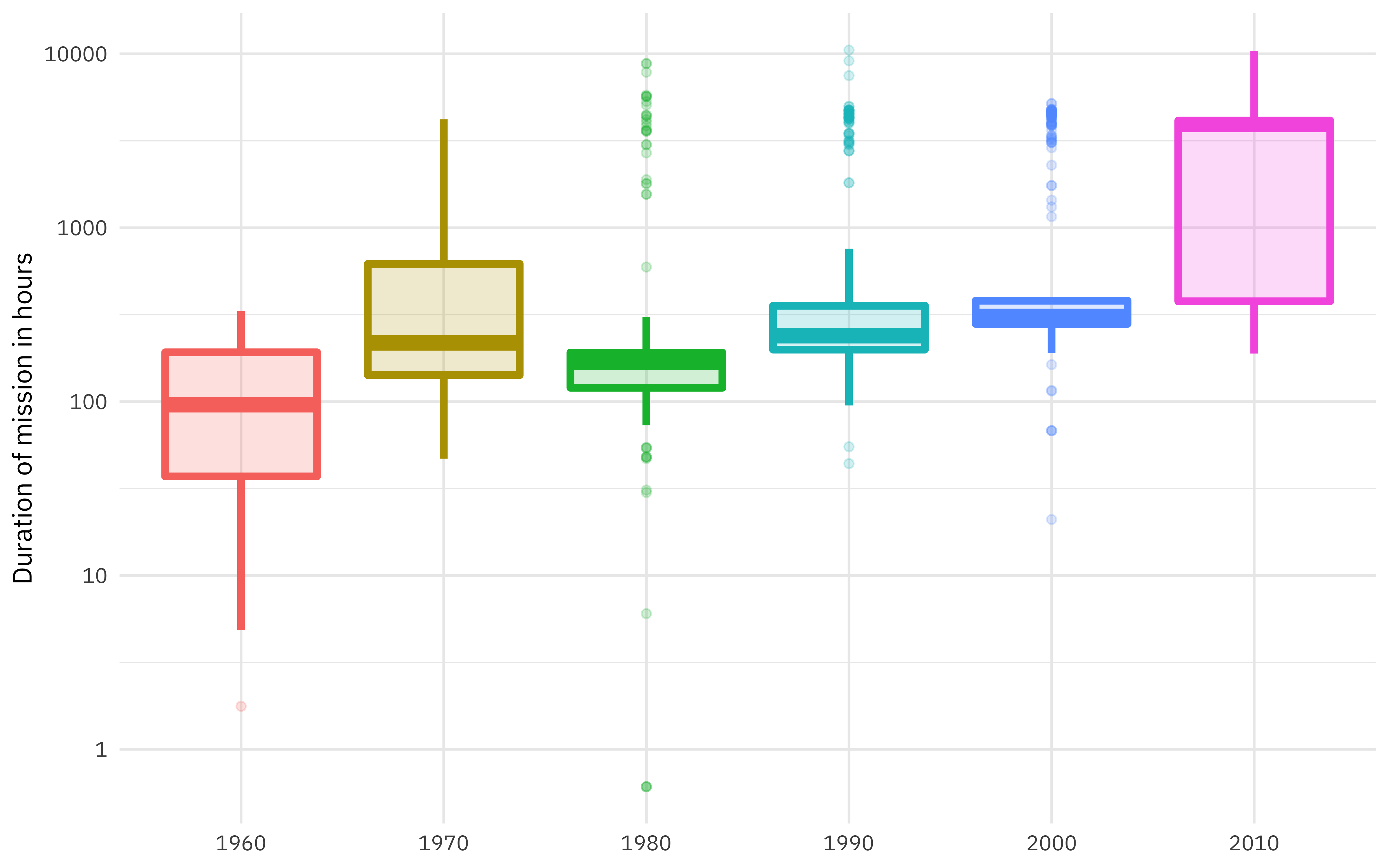
This duration is what we want to build a model to predict, using the other information in this per-astronaut-per-mission dataset. Let’s get ready for modeling next, by bucketing some of the spacecraft together (such as all the space shuttle missions) and taking the logarithm of the mission length.

astronauts_df <- astronauts %>%
  select(
    name, mission_title, hours_mission,
    military_civilian, occupation, year_of_mission, in_orbit
  ) %>%
  mutate(
    in_orbit = case_when(
      str_detect(in_orbit, "^Salyut") ~ "Salyut",
      str_detect(in_orbit, "^STS") ~ "STS",
      TRUE ~ in_orbit
    ),
    occupation = str_to_lower(occupation)
  ) %>%
  filter(hours_mission > 0) %>%
  mutate(hours_mission = log(hours_mission)) %>%
  na.omit()

It may make more sense to perform transformations like taking the logarithm of the outcome during data cleaning, before feature engineering and using any tidymodels packages like recipes. This kind of transformation is deterministic and can cause problems for tuning and resampling.

Build a model

We can start by loading the tidymodels metapackage, and splitting our data into training and testing sets.

library(tidymodels)

set.seed(123)
astro_split <- initial_split(astronauts_df, strata = hours_mission)
astro_train <- training(astro_split)
astro_test <- testing(astro_split)

Next, let’s preprocess our data to get it ready for modeling.

astro_recipe <- recipe(hours_mission ~ ., data = astro_train) %>%
  update_role(name, mission_title, new_role = "id") %>%
  step_other(occupation, in_orbit,
    threshold = 0.005, other = "Other"
  ) %>%
  step_dummy(all_nominal(), -has_role("id"))

Let’s walk through the steps in this recipe.

• First, we must tell the recipe() what our model is going to be (using a formula here) and what data we are using.
• Next, update the role for the two columns that are not predictors or outcome. This way, we can keep them in the data for identification later.
• There are a lot of different occupations and spacecraft in this dataset, so let’s collapse some of the less frequently occurring levels into an “Other” category, for each predictor.
• Finally, we can create indicator variables.

We’re going to use this recipe in a workflow() so we don’t need to stress about whether to prep() or not.

astro_wf <- workflow() %>%
  add_recipe(astro_recipe)

astro_wf

## ══ Workflow ════════════════════════════════════════════════════════════════════════════════════
## Preprocessor: Recipe
## Model: None
## 
## ── Preprocessor ────────────────────────────────────────────────────────────────────────────────
## 2 Recipe Steps
## 
## ● step_other()
## ● step_dummy()

For this analysis, we are going to build a bagging, i.e. bootstrap aggregating, model. This is an ensembling and model averaging method that:

• improves accuracy and stability
• reduces overfitting and variance

In tidymodels, you can create bagging ensemble models with baguette, a parsnip-adjacent package. The baguette functions create new bootstrap training sets by sampling with replacement and then fit a model to each new training set. These models are combined by averaging the predictions for the regression case, like what we have here (by voting, for classification).

Let’s make two bagged models, one with decision trees and one with MARS models.

library(baguette)

tree_spec <- bag_tree() %>%
  set_engine("rpart", times = 25) %>%
  set_mode("regression")

tree_spec

## Bagged Decision Tree Model Specification (regression)
## 
## Main Arguments:
##   cost_complexity = 0
##   min_n = 2
## 
## Engine-Specific Arguments:
##   times = 25
## 
## Computational engine: rpart

mars_spec <- bag_mars() %>%
  set_engine("earth", times = 25) %>%
  set_mode("regression")

mars_spec

## Bagged MARS Model Specification (regression)
## 
## Engine-Specific Arguments:
##   times = 25
## 
## Computational engine: earth

Let’s fit these models to the training data.

tree_rs <- astro_wf %>%
  add_model(tree_spec) %>%
  fit(astro_train)

tree_rs

## ══ Workflow [trained] ══════════════════════════════════════════════════════════════════════════
## Preprocessor: Recipe
## Model: bag_tree()
## 
## ── Preprocessor ────────────────────────────────────────────────────────────────────────────────
## 2 Recipe Steps
## 
## ● step_other()
## ● step_dummy()
## 
## ── Model ───────────────────────────────────────────────────────────────────────────────────────
## Bagged CART (regression with 25 members)
## 
## Variable importance scores include:
## 
## # A tibble: 11 x 4
##    term                       value std.error  used
##    <chr>                      <dbl>     <dbl> <int>
##  1 year_of_mission            890.      18.5     25
##  2 in_orbit_Other             689.      55.6     25
##  3 in_orbit_STS               386.      19.4     25
##  4 occupation_flight.engineer 190.      14.9     25
##  5 occupation_pilot           189.      20.4     25
##  6 in_orbit_Mir               124.      20.7     25
##  7 in_orbit_Salyut            100.       9.61    25
##  8 occupation_MSP              96.3      9.89    25
##  9 occupation_Other            54.7      4.09    25
## 10 military_civilian_military  39.8      4.77    25
## 11 occupation_PSP              34.4      6.24    25

mars_rs <- astro_wf %>%
  add_model(mars_spec) %>%
  fit(astro_train)

mars_rs

## ══ Workflow [trained] ══════════════════════════════════════════════════════════════════════════
## Preprocessor: Recipe
## Model: bag_mars()
## 
## ── Preprocessor ────────────────────────────────────────────────────────────────────────────────
## 2 Recipe Steps
## 
## ● step_other()
## ● step_dummy()
## 
## ── Model ───────────────────────────────────────────────────────────────────────────────────────
## Bagged MARS (regression with 25 members)
## 
## Variable importance scores include:
## 
## # A tibble: 10 x 4
##    term                         value std.error  used
##    <chr>                        <dbl>     <dbl> <int>
##  1 in_orbit_STS               100         0        25
##  2 in_orbit_Other              91.7       1.78     25
##  3 year_of_mission             62.6       4.46     25
##  4 in_orbit_Salyut             31.7       2.41     25
##  5 in_orbit_Mir                 1.08      0.914     4
##  6 military_civilian_military   0.699     1.43      2
##  7 occupation_Other             0.698     0.186     3
##  8 occupation_PSP               0.542     0.924     2
##  9 occupation_pilot             0.436     0.710     2
## 10 occupation_flight.engineer   0.215     0         1

The models return aggregated variable importance scores, and we can see that the spacecraft and year are importance in both models.

Evaluate model

Let’s evaluate how well these two models did by evaluating performance on the test data.

test_rs <- astro_test %>%
  bind_cols(predict(tree_rs, astro_test)) %>%
  rename(.pred_tree = .pred) %>%
  bind_cols(predict(mars_rs, astro_test)) %>%
  rename(.pred_mars = .pred)

test_rs

## # A tibble: 316 x 9
##    name  mission_title hours_mission military_civili… occupation year_of_mission
##    <chr> <chr>                 <dbl> <chr>            <chr>                <dbl>
##  1 Carp… Mercury-Atla…          1.61 military         Pilot                 1962
##  2 Schi… Mercury-Atla…          2.22 military         pilot                 1962
##  3 Tere… Vostok 6               4.26 military         pilot                 1963
##  4 Koma… Voskhod 1              3.19 military         commander             1964
##  5 Feok… Voskhod 1              3.19 civilian         MSP                   1964
##  6 Youn… Gemini 10              4.26 military         pilot                 1966
##  7 Youn… Apollo 16              5.58 military         commander             1972
##  8 Youn… STS-9                  5.48 military         commander             1983
##  9 McDi… Gemini 4               4.57 military         commander             1965
## 10 Whit… Gemini 4               4.58 military         pilot                 1965
## # … with 306 more rows, and 3 more variables: in_orbit <chr>, .pred_tree <dbl>,
## #   .pred_mars <dbl>

We can use the metrics() function from yardstick for both sets of predictions.

test_rs %>%
  metrics(hours_mission, .pred_tree)

## # A tibble: 3 x 3
##   .metric .estimator .estimate
##   <chr>   <chr>          <dbl>
## 1 rmse    standard       0.640
## 2 rsq     standard       0.798
## 3 mae     standard       0.357

test_rs %>%
  metrics(hours_mission, .pred_mars)

## # A tibble: 3 x 3
##   .metric .estimator .estimate
##   <chr>   <chr>          <dbl>
## 1 rmse    standard       0.640
## 2 rsq     standard       0.795
## 3 mae     standard       0.351

Both models performed pretty similarly.

Let’s make some “new” astronauts to understand the kinds of predictions our bagged tree model is making.

new_astronauts <- crossing(
  in_orbit = fct_inorder(c("ISS", "STS", "Mir", "Other")),
  military_civilian = "civilian",
  occupation = "Other",
  year_of_mission = seq(1960, 2020, by = 10),
  name = "id", mission_title = "id"
) %>%
  filter(
    !(in_orbit == "ISS" & year_of_mission < 2000),
    !(in_orbit == "Mir" & year_of_mission < 1990),
    !(in_orbit == "STS" & year_of_mission > 2010),
    !(in_orbit == "STS" & year_of_mission < 1980)
  )

new_astronauts

## # A tibble: 18 x 6
##    in_orbit military_civilian occupation year_of_mission name  mission_title
##    <fct>    <chr>             <chr>                <dbl> <chr> <chr>        
##  1 ISS      civilian          Other                 2000 id    id           
##  2 ISS      civilian          Other                 2010 id    id           
##  3 ISS      civilian          Other                 2020 id    id           
##  4 STS      civilian          Other                 1980 id    id           
##  5 STS      civilian          Other                 1990 id    id           
##  6 STS      civilian          Other                 2000 id    id           
##  7 STS      civilian          Other                 2010 id    id           
##  8 Mir      civilian          Other                 1990 id    id           
##  9 Mir      civilian          Other                 2000 id    id           
## 10 Mir      civilian          Other                 2010 id    id           
## 11 Mir      civilian          Other                 2020 id    id           
## 12 Other    civilian          Other                 1960 id    id           
## 13 Other    civilian          Other                 1970 id    id           
## 14 Other    civilian          Other                 1980 id    id           
## 15 Other    civilian          Other                 1990 id    id           
## 16 Other    civilian          Other                 2000 id    id           
## 17 Other    civilian          Other                 2010 id    id           
## 18 Other    civilian          Other                 2020 id    id

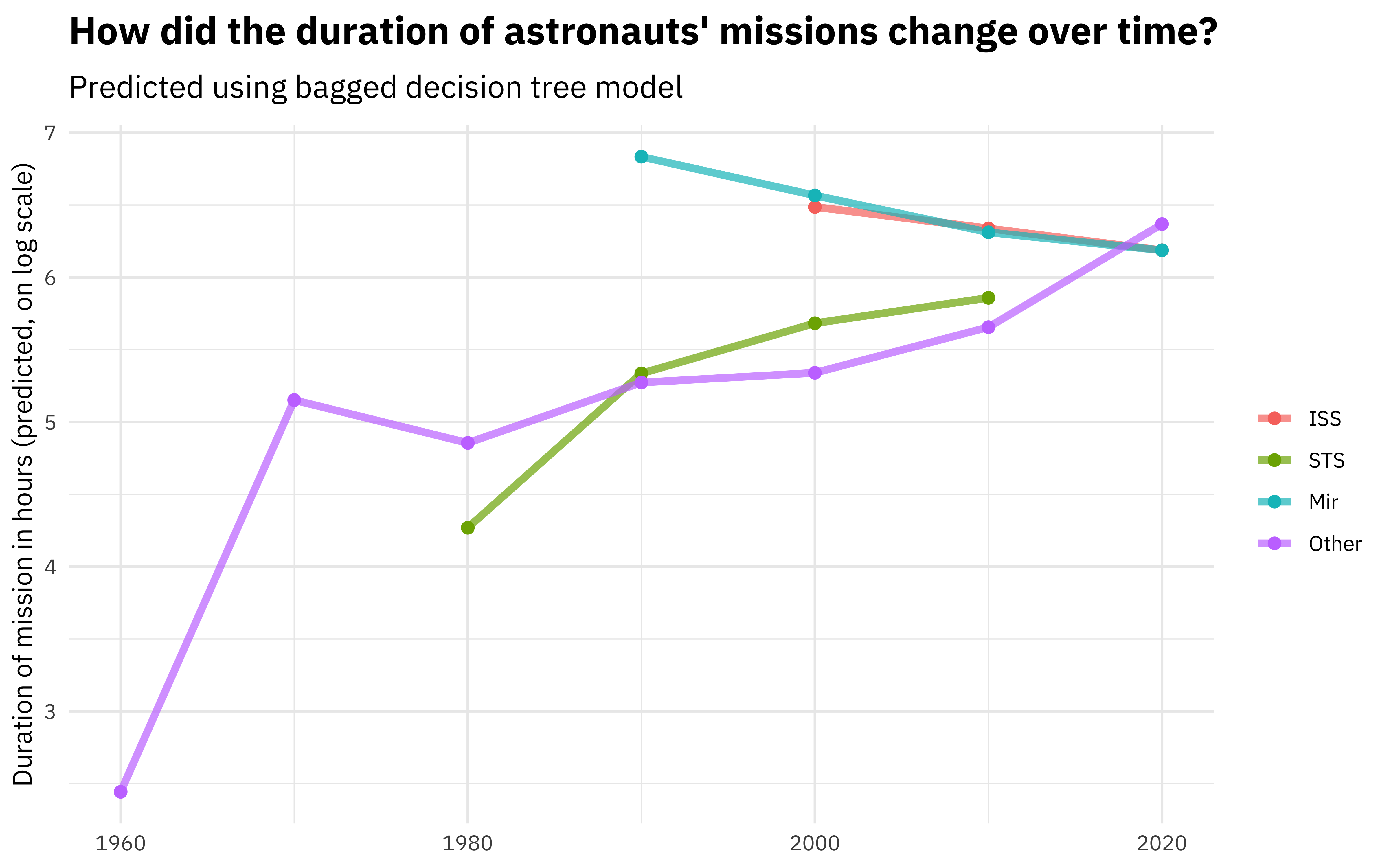
Let’s start with the decision tree model.

new_astronauts %>%
  bind_cols(predict(tree_rs, new_astronauts)) %>%
  ggplot(aes(year_of_mission, .pred, color = in_orbit)) +
  geom_line(size = 1.5, alpha = 0.7) +
  geom_point(size = 2) +
  labs(
    x = NULL, y = "Duration of mission in hours (predicted, on log scale)",
    color = NULL, title = "How did the duration of astronauts' missions change over time?",
    subtitle = "Predicted using bagged decision tree model"
  )

What about the MARS model?

new_astronauts %>%
  bind_cols(predict(mars_rs, new_astronauts)) %>%
  ggplot(aes(year_of_mission, .pred, color = in_orbit)) +
  geom_line(size = 1.5, alpha = 0.7) +
  geom_point(size = 2) +
  labs(
    x = NULL, y = "Duration of mission in hours (predicted, on log scale)",
    color = NULL, title = "How did the duration of astronauts' missions change over time?",
    subtitle = "Predicted using bagged MARS model"
  )

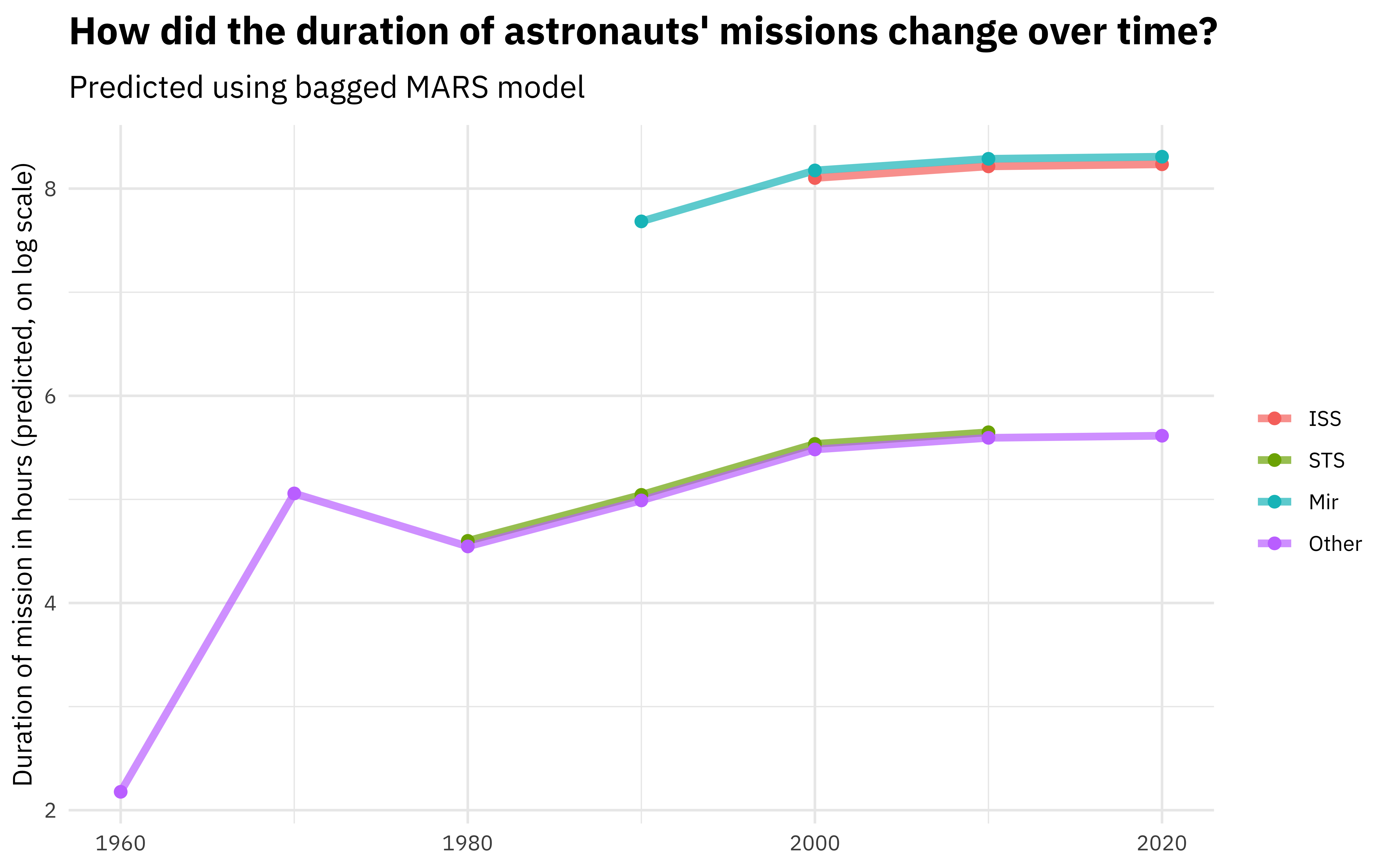
You can really get a sense of how these two kinds of models work from the differences in these plots (tree vs. splines with knots), but from both, we can see that missions to space stations are longer, and missions in that “Other” category change characteristics over time pretty dramatically.