Predicting injuries for Chicago traffic crashes
By Julia Silge in rstats tidymodels
January 4, 2021
This is the latest in my series of screencasts demonstrating how to use the tidymodels packages, from starting out with first modeling steps to tuning more complex models. Instead of Tidy Tuesday data, this screencast uses some “wild caught” data from Chicago’s open data portal and is planned to be the first in a series walking through how to approach model ops tasks using tidymodels and other R tools. This screencast focuses on training a model, for traffic crashes in Chicago. We can build a model to predict whether a crash involved an injury or not. 🚗
Here is the code I used in the video, for those who prefer reading instead of or in addition to video.
Explore data
This dataset covers traffic crashes on city streets within Chicago city limits under the jurisdiction of the Chicago Police Department.
Let’s download the last two years of data to train our model.
library(tidyverse)
library(lubridate)
library(RSocrata)

years_ago <- today() - years(2)
crash_url <- glue::glue("https://data.cityofchicago.org/Transportation/Traffic-Crashes-Crashes/85ca-t3if?$where=CRASH_DATE > '{years_ago}'")
crash_raw <- as_tibble(read.socrata(crash_url))

crash <- crash_raw %>%
  arrange(desc(crash_date)) %>%
  transmute(
    injuries = if_else(injuries_total > 0, "injuries", "none"),
    crash_date,
    crash_hour,
    report_type = if_else(report_type == "", "UNKNOWN", report_type),
    num_units,
    posted_speed_limit,
    weather_condition,
    lighting_condition,
    roadway_surface_cond,
    first_crash_type,
    trafficway_type,
    prim_contributory_cause,
    latitude, longitude
  ) %>%
  na.omit()

crash
## # A tibble: 207,422 x 14
##    injuries crash_date          crash_hour report_type num_units
##    <chr>    <dttm>                   <int> <chr>           <int>
##  1 none     2021-01-03 03:00:00          3 ON SCENE            3
##  2 none     2021-01-03 01:37:00          1 ON SCENE            1
##  3 none     2021-01-03 01:25:00          1 ON SCENE            2
##  4 none     2021-01-03 01:01:00          1 ON SCENE            2
##  5 injuries 2021-01-03 00:45:00          0 ON SCENE            2
##  6 injuries 2021-01-03 00:10:00          0 ON SCENE            2
##  7 none     2021-01-03 00:10:00          0 NOT ON SCE…         2
##  8 none     2021-01-02 23:30:00         23 NOT ON SCE…         2
##  9 injuries 2021-01-02 22:46:00         22 NOT ON SCE…         2
## 10 none     2021-01-02 22:40:00         22 ON SCENE            2
## # … with 207,412 more rows, and 9 more variables: posted_speed_limit <int>,
## #   weather_condition <chr>, lighting_condition <chr>,
## #   roadway_surface_cond <chr>, first_crash_type <chr>, trafficway_type <chr>,
## #   prim_contributory_cause <chr>, latitude <dbl>, longitude <dbl>
How have the number of crashes changed over time?
crash %>%
  mutate(crash_date = floor_date(crash_date, unit = "week")) %>%
  count(crash_date, injuries) %>%
  filter(
    crash_date != last(crash_date),
    crash_date != first(crash_date)
  ) %>%
  ggplot(aes(crash_date, n, color = injuries)) +
  geom_line(size = 1.5, alpha = 0.7) +
  scale_y_continuous(limits = (c(0, NA))) +
  labs(
    x = NULL, y = "Number of traffic crashes per week",
    color = "Injuries?"
  )
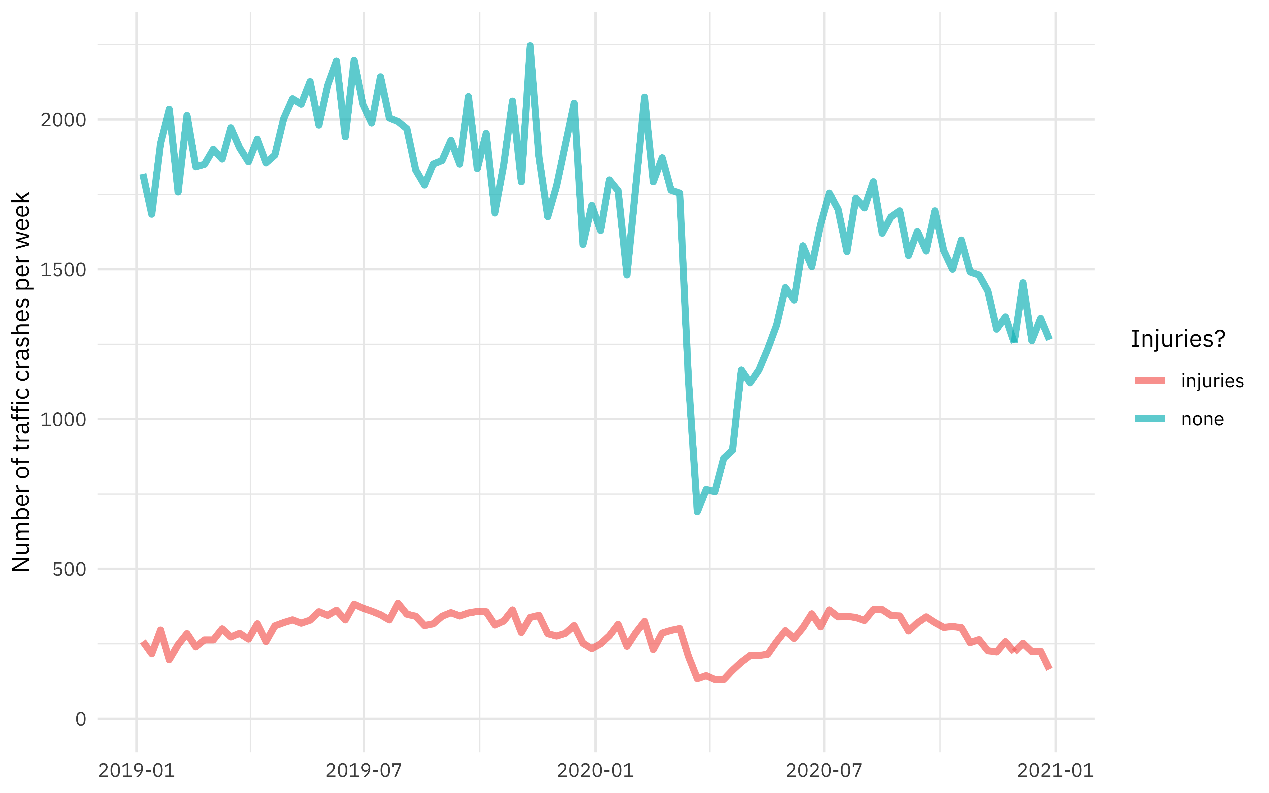
WOW, look at the impact of the global pandemic during 2020! 😮
How has the injury rate changed over time?
crash %>%
  mutate(crash_date = floor_date(crash_date, unit = "week")) %>%
  count(crash_date, injuries) %>%
  filter(
    crash_date != last(crash_date),
    crash_date != first(crash_date)
  ) %>%
  group_by(crash_date) %>%
  mutate(percent_injury = n / sum(n)) %>%
  ungroup() %>%
  filter(injuries == "injuries") %>%
  ggplot(aes(crash_date, percent_injury)) +
  geom_line(size = 1.5, alpha = 0.7, color = "midnightblue") +
  scale_y_continuous(limits = c(0, NA), labels = percent_format()) +
  labs(x = NULL, y = "% of crashes that involve injuries")
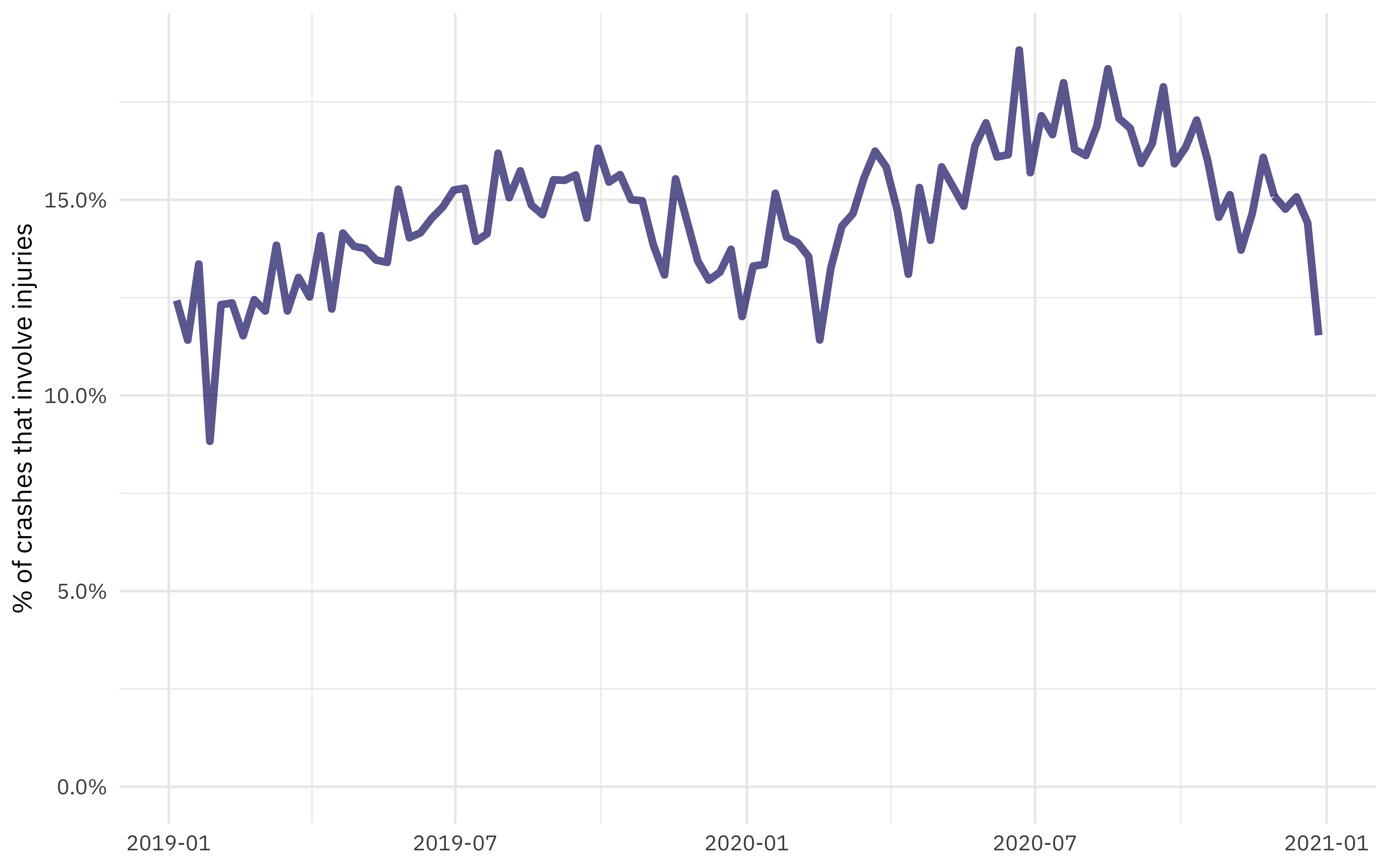
This is the kind of data drift or concept drift that becomes important for model monitoring, where we are headed with this model!
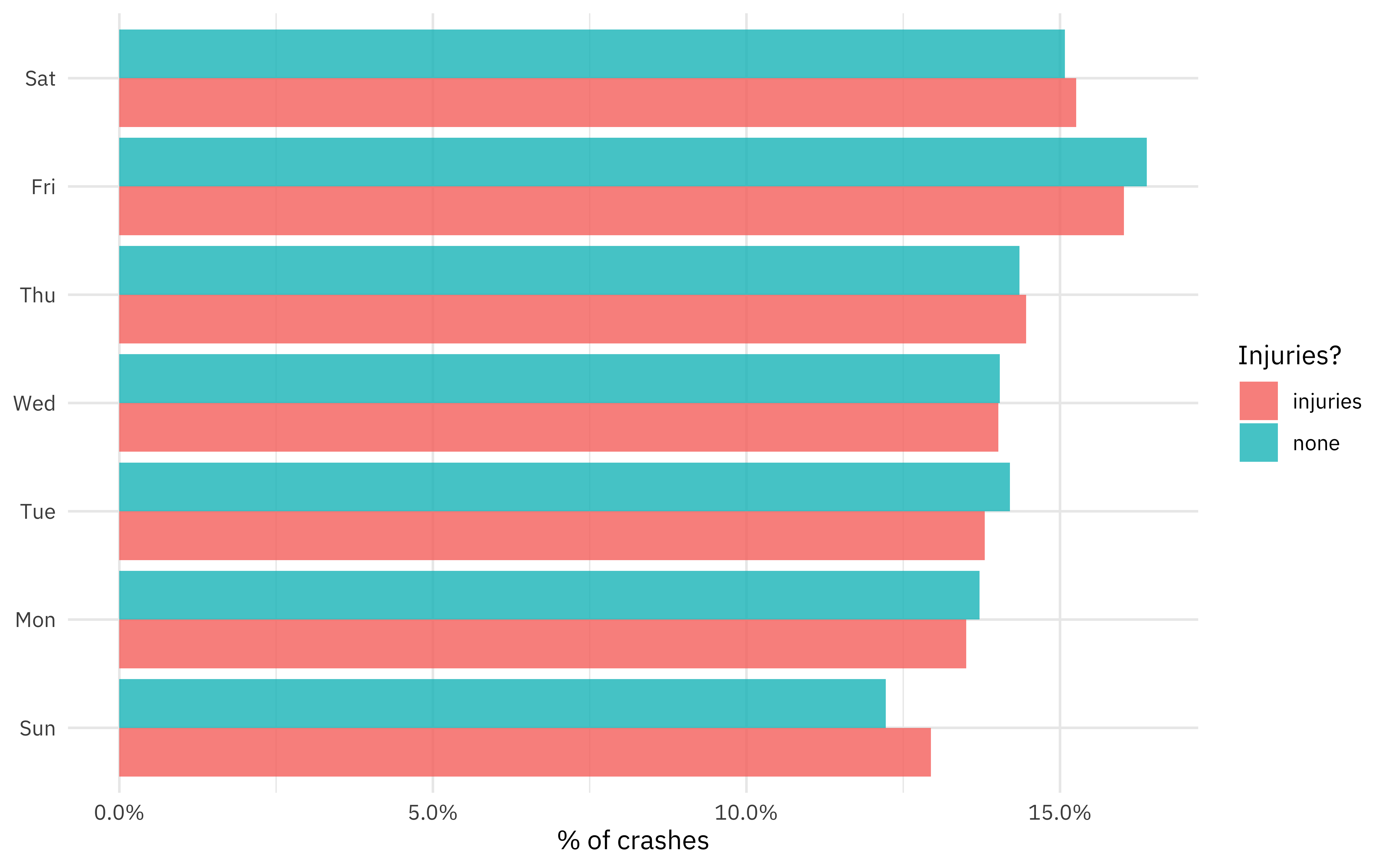
How does the injury rate change through the week?
crash %>%
  mutate(crash_date = wday(crash_date, label = TRUE)) %>%
  count(crash_date, injuries) %>%
  group_by(injuries) %>%
  mutate(percent = n / sum(n)) %>%
  ungroup() %>%
  ggplot(aes(percent, crash_date, fill = injuries)) +
  geom_col(position = "dodge", alpha = 0.8) +
  scale_x_continuous(labels = percent_format()) +
  labs(x = "% of crashes", y = NULL, fill = "Injuries?")
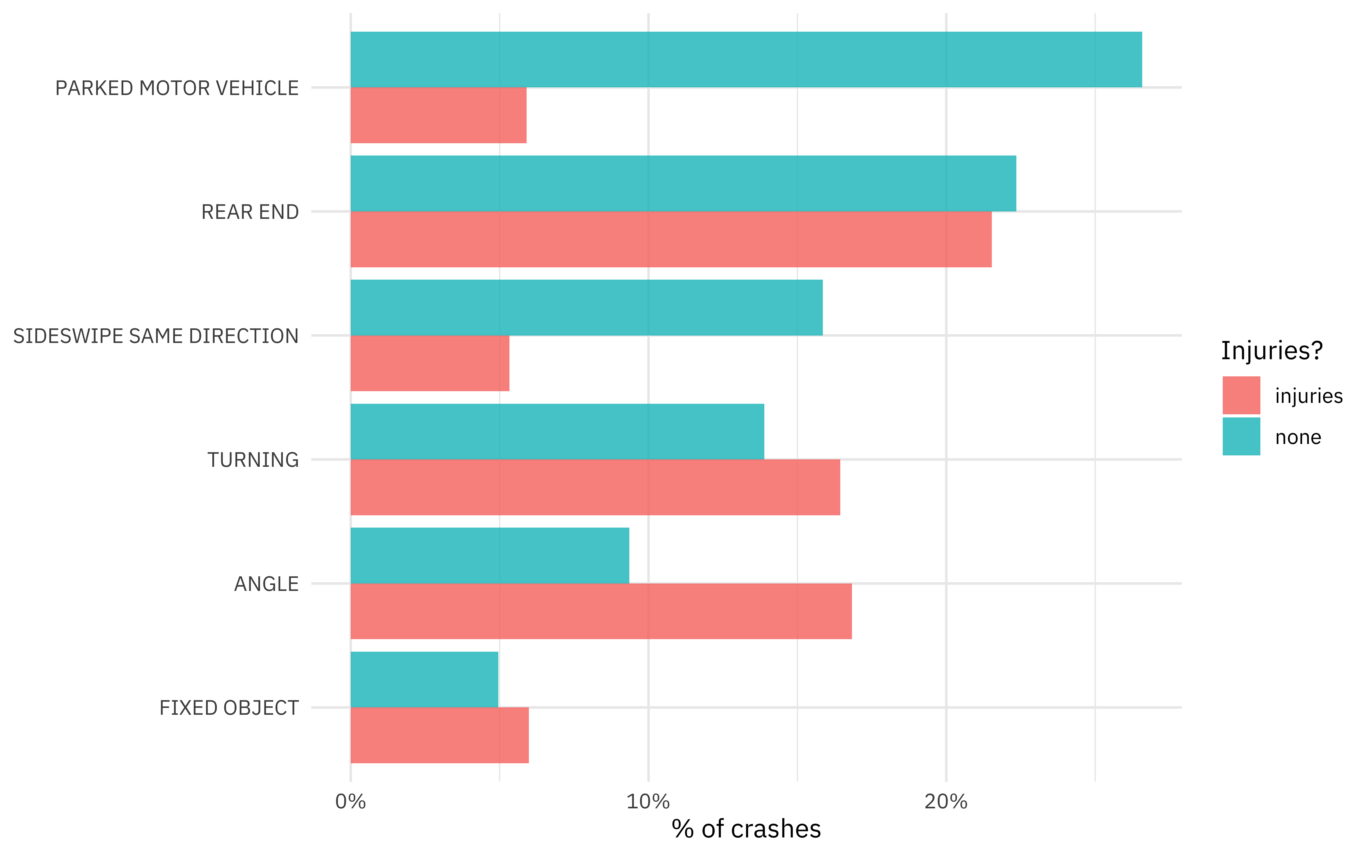
How do injuries vary with first crash type?
crash %>%
  count(first_crash_type, injuries) %>%
  mutate(first_crash_type = fct_reorder(first_crash_type, n)) %>%
  group_by(injuries) %>%
  mutate(percent = n / sum(n)) %>%
  ungroup() %>%
  group_by(first_crash_type) %>%
  filter(sum(n) > 1e4) %>%
  ungroup() %>%
  ggplot(aes(percent, first_crash_type, fill = injuries)) +
  geom_col(position = "dodge", alpha = 0.8) +
  scale_x_continuous(labels = percent_format()) +
  labs(x = "% of crashes", y = NULL, fill = "Injuries?")
Are injuries more likely in different locations?
crash %>%
  filter(latitude > 0) %>%
  ggplot(aes(longitude, latitude, color = injuries)) +
  geom_point(size = 0.5, alpha = 0.4) +
  labs(color = NULL) +
  scale_color_manual(values = c("deeppink4", "gray80")) +
  coord_fixed()
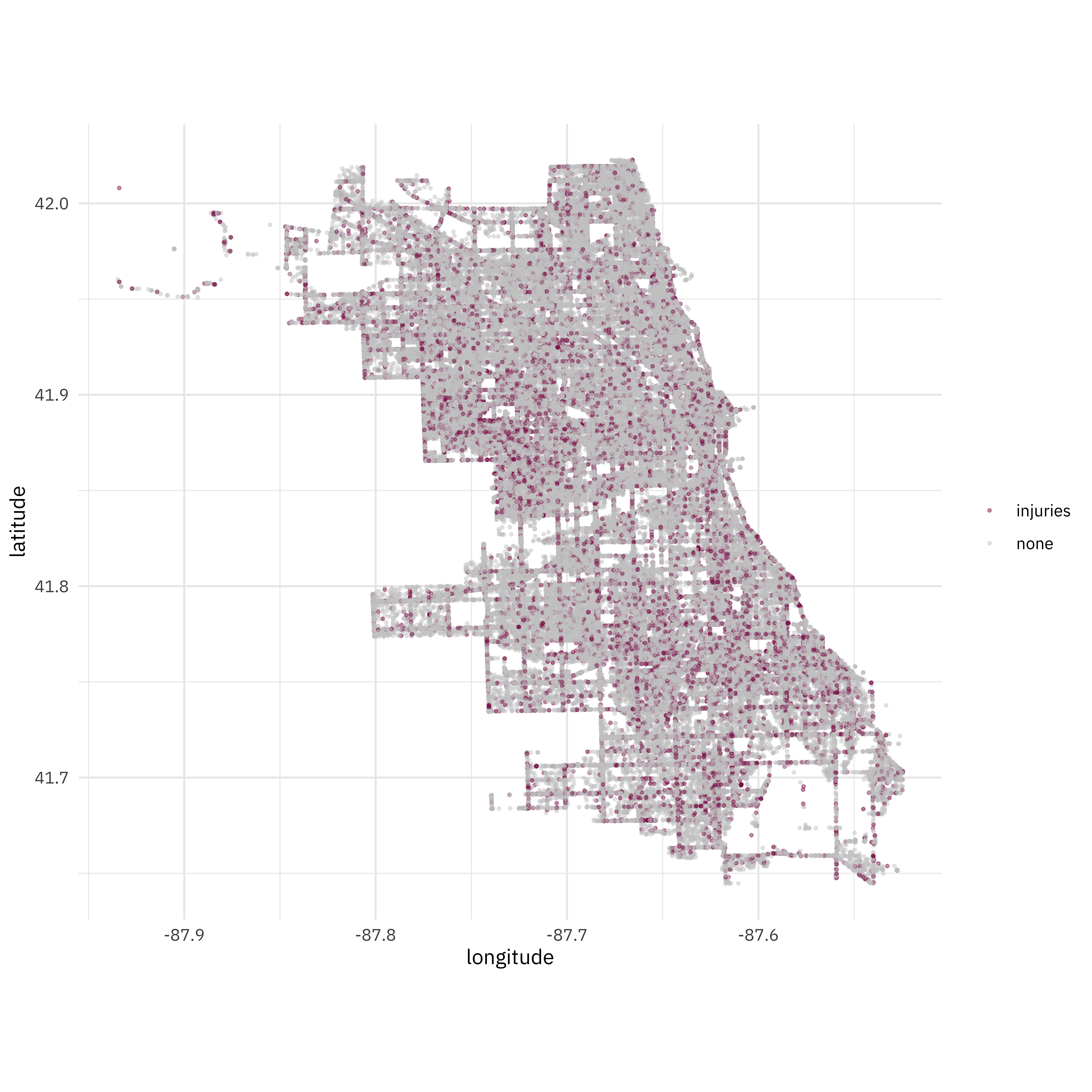
This is all the information we will use in building our model to predict which crashes caused injuries.
Build a model
Let’s start by splitting our data and creating cross-validation folds.
library(tidymodels)

set.seed(2020)
crash_split <- initial_split(crash, strata = injuries)
crash_train <- training(crash_split)
crash_test <- testing(crash_split)

set.seed(123)
crash_folds <- vfold_cv(crash_train, strata = injuries)
crash_folds
## #  10-fold cross-validation using stratification
## # A tibble: 10 x 2
##    splits               id
##    <list>               <chr>
##  1 <split [140K/15.6K]> Fold01
##  2 <split [140K/15.6K]> Fold02
##  3 <split [140K/15.6K]> Fold03
##  4 <split [140K/15.6K]> Fold04
##  5 <split [140K/15.6K]> Fold05
##  6 <split [140K/15.6K]> Fold06
##  7 <split [140K/15.6K]> Fold07
##  8 <split [140K/15.6K]> Fold08
##  9 <split [140K/15.6K]> Fold09
## 10 <split [140K/15.6K]> Fold10
Next, let’s create a model.
- The feature engineering includes creating date features such as day of the week, handling the high cardinality of weather conditions, contributing cause, etc, and perhaps most importantly, downsampling to account for the class imbalance (injuries are more rare than non-injury-causing crashes).
- After experimenting with random forests and xgboost, this smaller bagged tree model achieved very nearly the same performance with a much smaller model “footprint” in terms of model size and prediction time.
library(themis)
library(baguette)

crash_rec <- recipe(injuries ~ ., data = crash_train) %>%
  step_date(crash_date) %>%
  step_rm(crash_date) %>%
  step_other(weather_condition, first_crash_type,
    trafficway_type, prim_contributory_cause,
    other = "OTHER"
  ) %>%
  step_downsample(injuries)

bag_spec <- bag_tree(min_n = 10) %>%
  set_engine("rpart", times = 25) %>%
  set_mode("classification")

crash_wf <- workflow() %>%
  add_recipe(crash_rec) %>%
  add_model(bag_spec)

crash_wf
## ══ Workflow ════════════════════════════════════════════════════════════════════
## Preprocessor: Recipe
## Model: bag_tree()
##
## ── Preprocessor ────────────────────────────────────────────────────────────────
## 4 Recipe Steps
##
## ● step_date()
## ● step_rm()
## ● step_other()
## ● step_downsample()
##
## ── Model ───────────────────────────────────────────────────────────────────────
## Bagged Decision Tree Model Specification (classification)
##
## Main Arguments:
##   cost_complexity = 0
##   min_n = 10
##
## Engine-Specific Arguments:
##   times = 25
##
## Computational engine: rpart
Let’s fit this model to the cross-validation resamples to understand how well it will perform.
doParallel::registerDoParallel()
crash_res <- fit_resamples(
  crash_wf,
  crash_folds,
  control = control_resamples(save_pred = TRUE)
)
Evaluate model
What do the results look like?
collect_metrics(crash_res)
## # A tibble: 2 x 6
##   .metric  .estimator  mean     n  std_err .config
##   <chr>    <chr>      <dbl> <int>    <dbl> <chr>
## 1 accuracy binary     0.727    10 0.00136  Preprocessor1_Model1
## 2 roc_auc  binary     0.819    10 0.000788 Preprocessor1_Model1
This is almost exactly what we achieved with models like random forest and xgboost, and looks to be about as good as we can do with this data.
Let’s now fit to the entire training set and evaluate on the testing set.
crash_fit <- last_fit(crash_wf, crash_split)
collect_metrics(crash_fit)
## # A tibble: 2 x 4
##   .metric  .estimator .estimate .config
##   <chr>    <chr>          <dbl> <chr>
## 1 accuracy binary         0.725 Preprocessor1_Model1
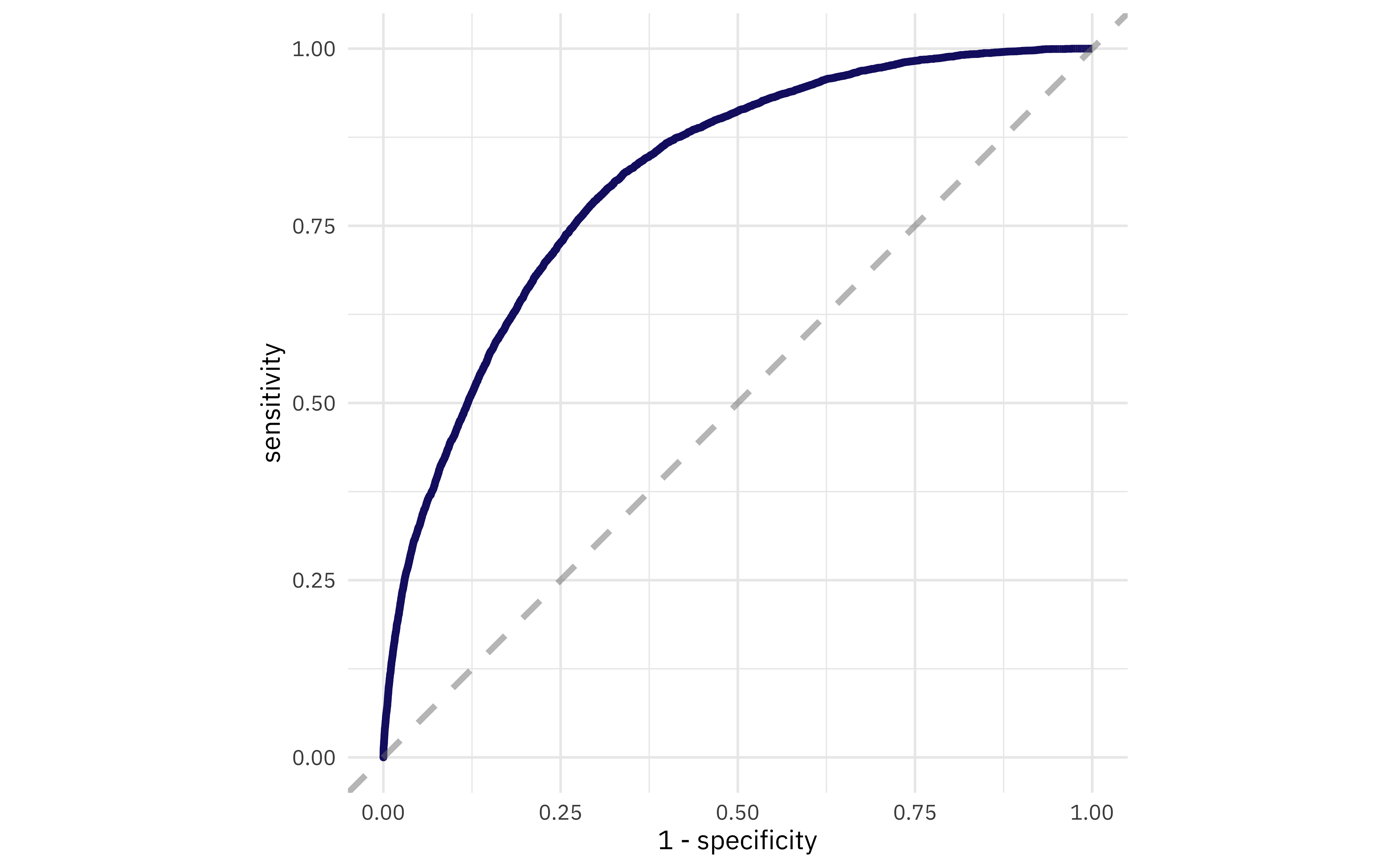
## 2 roc_auc  binary         0.817 Preprocessor1_Model1
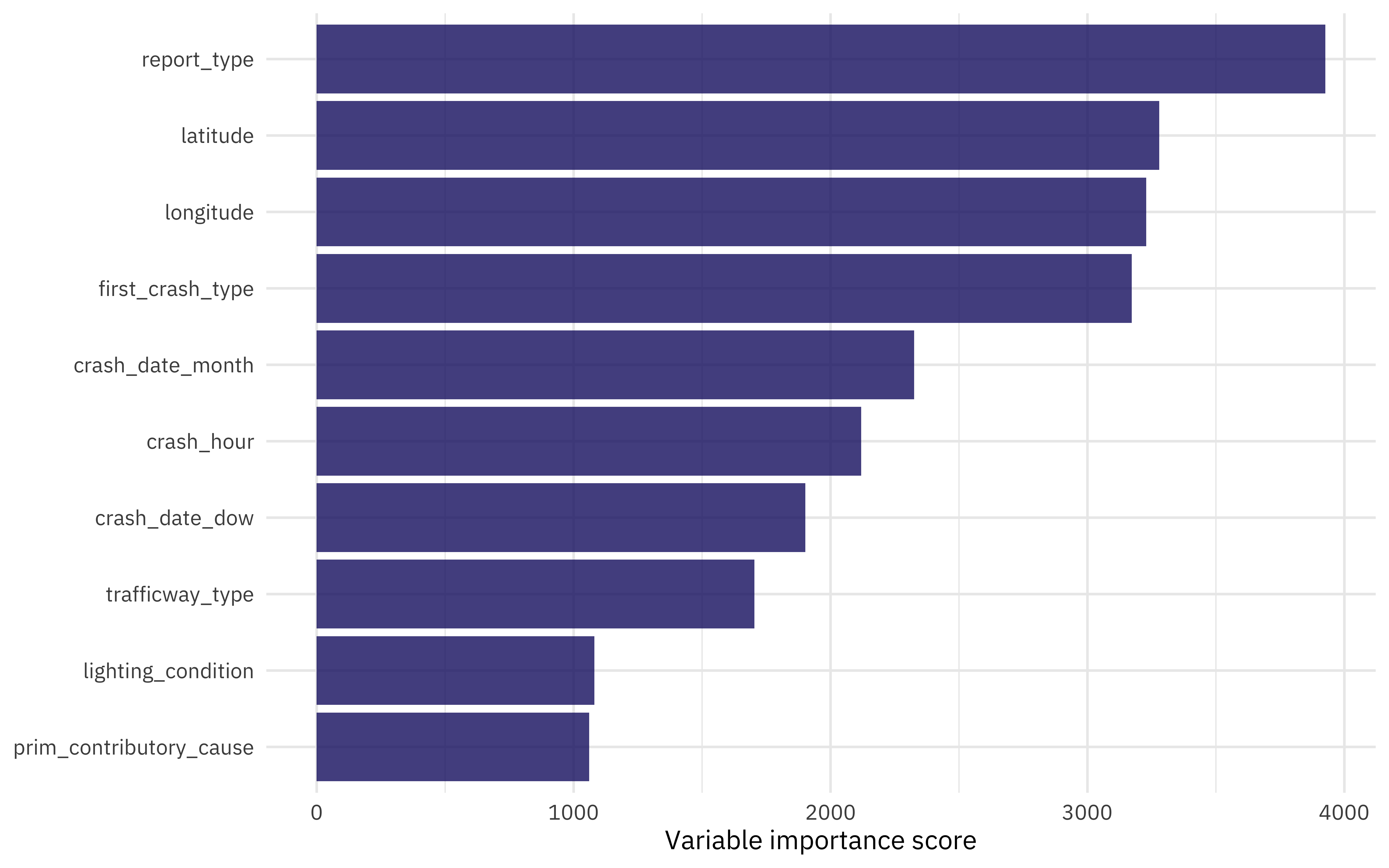
Which features were most important in predicting an injury?
crash_imp <- crash_fit$.workflow[[1]] %>%
  pull_workflow_fit()

crash_imp$fit$imp %>%
  slice_max(value, n = 10) %>%
  ggplot(aes(value, fct_reorder(term, value))) +
  geom_col(alpha = 0.8, fill = "midnightblue") +
  labs(x = "Variable importance score", y = NULL)
How does the ROC curve for the testing data look?
collect_predictions(crash_fit) %>%
  roc_curve(injuries, .pred_injuries) %>%
  ggplot(aes(x = 1 - specificity, y = sensitivity)) +
  geom_line(size = 1.5, color = "midnightblue") +
  geom_abline(
    lty = 2, alpha = 0.5,
    color = "gray50",
    size = 1.2
  ) +
  coord_equal()
Save model
I am happy with this model, so we need to save (serialize) it to be used in our model API.
crash_wf_model <- crash_fit$.workflow[[1]]
This is an object we can make predictions with. Is this particular crash predicted to have any injuries?
predict(crash_wf_model, crash_test[222, ])
## # A tibble: 1 x 1
##   .pred_class
##   <fct>
## 1 none
Now let’s save this model and the metrics to be used later in our model.
saveRDS(crash_wf_model, here::here("crash-api", "crash-wf-model.rds"))

collect_metrics(crash_res) %>%
  write_csv(here::here("crash-api", "crash-model-metrics.csv"))
Look for more soon on how to publish this model as an API and how to monitor its performance!
- Posted on:
- January 4, 2021
- Length:
- 7 minute read, 1336 words
- Categories:
- rstats tidymodels
- Tags:
- rstats tidymodels