Tune an xgboost model with early stopping and #TidyTuesday childcare costs

This is the latest in my series of screencasts! This screencast focuses on how to use tidymodels to tune an xgboost model with early stopping, using this week’s #TidyTuesday dataset on childcare costs in the United States. 👩‍👧‍👦

Here is the code I used in the video, for those who prefer reading instead of or in addition to video.

Explore data

Mothers Day is coming up this weekend, and our modeling goal in this case is to predict the cost of childcare in US counties based on other characteristics of each county, like the poverty rate and labor force participation. Let’s start by reading in the data:

library(tidyverse)

childcare_costs <- read_csv('https://raw.githubusercontent.com/rfordatascience/tidytuesday/master/data/2023/2023-05-09/childcare_costs.csv')

glimpse(childcare_costs)

## Rows: 34,567
## Columns: 61
## $ county_fips_code          <dbl> 1001, 1001, 1001, 1001, 1001, 1001, 1001, 10…
## $ study_year                <dbl> 2008, 2009, 2010, 2011, 2012, 2013, 2014, 20…
## $ unr_16                    <dbl> 5.42, 5.93, 6.21, 7.55, 8.60, 9.39, 8.50, 7.…
## $ funr_16                   <dbl> 4.41, 5.72, 5.57, 8.13, 8.88, 10.31, 9.18, 8…
## $ munr_16                   <dbl> 6.32, 6.11, 6.78, 7.03, 8.29, 8.56, 7.95, 6.…
## $ unr_20to64                <dbl> 4.6, 4.8, 5.1, 6.2, 6.7, 7.3, 6.8, 5.9, 4.4,…
## $ funr_20to64               <dbl> 3.5, 4.6, 4.6, 6.3, 6.4, 7.6, 6.8, 6.1, 4.6,…
## $ munr_20to64               <dbl> 5.6, 5.0, 5.6, 6.1, 7.0, 7.0, 6.8, 5.9, 4.3,…
## $ flfpr_20to64              <dbl> 68.9, 70.8, 71.3, 70.2, 70.6, 70.7, 69.9, 68…
## $ flfpr_20to64_under6       <dbl> 66.9, 63.7, 67.0, 66.5, 67.1, 67.5, 65.2, 66…
## $ flfpr_20to64_6to17        <dbl> 79.59, 78.41, 78.15, 77.62, 76.31, 75.91, 75…
## $ flfpr_20to64_under6_6to17 <dbl> 60.81, 59.91, 59.71, 59.31, 58.30, 58.00, 57…
## $ mlfpr_20to64              <dbl> 84.0, 86.2, 85.8, 85.7, 85.7, 85.0, 84.2, 82…
## $ pr_f                      <dbl> 8.5, 7.5, 7.5, 7.4, 7.4, 8.3, 9.1, 9.3, 9.4,…
## $ pr_p                      <dbl> 11.5, 10.3, 10.6, 10.9, 11.6, 12.1, 12.8, 12…
## $ mhi_2018                  <dbl> 58462.55, 60211.71, 61775.80, 60366.88, 5915…
## $ me_2018                   <dbl> 32710.60, 34688.16, 34740.84, 34564.32, 3432…
## $ fme_2018                  <dbl> 25156.25, 26852.67, 27391.08, 26727.68, 2796…
## $ mme_2018                  <dbl> 41436.80, 43865.64, 46155.24, 45333.12, 4427…
## $ total_pop                 <dbl> 49744, 49584, 53155, 53944, 54590, 54907, 55…
## $ one_race                  <dbl> 98.1, 98.6, 98.5, 98.5, 98.5, 98.6, 98.7, 98…
## $ one_race_w                <dbl> 78.9, 79.1, 79.1, 78.9, 78.9, 78.3, 78.0, 77…
## $ one_race_b                <dbl> 17.7, 17.9, 17.9, 18.1, 18.1, 18.4, 18.6, 18…
## $ one_race_i                <dbl> 0.4, 0.4, 0.3, 0.2, 0.3, 0.3, 0.4, 0.4, 0.4,…
## $ one_race_a                <dbl> 0.4, 0.6, 0.7, 0.7, 0.8, 1.0, 0.9, 1.0, 0.8,…
## $ one_race_h                <dbl> 0.0, 0.0, 0.0, 0.0, 0.0, 0.0, 0.0, 0.0, 0.1,…
## $ one_race_other            <dbl> 0.7, 0.7, 0.6, 0.5, 0.4, 0.7, 0.7, 0.9, 1.4,…
## $ two_races                 <dbl> 1.9, 1.4, 1.5, 1.5, 1.5, 1.4, 1.3, 1.6, 2.0,…
## $ hispanic                  <dbl> 1.8, 2.0, 2.3, 2.4, 2.4, 2.5, 2.5, 2.6, 2.6,…
## $ households                <dbl> 18373, 18288, 19718, 19998, 19934, 20071, 20…
## $ h_under6_both_work        <dbl> 1543, 1475, 1569, 1695, 1714, 1532, 1557, 13…
## $ h_under6_f_work           <dbl> 970, 964, 1009, 1060, 938, 880, 1191, 1258, …
## $ h_under6_m_work           <dbl> 22, 16, 16, 106, 120, 161, 159, 211, 109, 10…
## $ h_under6_single_m         <dbl> 995, 1099, 1110, 1030, 1095, 1160, 954, 883,…
## $ h_6to17_both_work         <dbl> 4900, 5028, 5472, 5065, 4608, 4238, 4056, 40…
## $ h_6to17_fwork             <dbl> 1308, 1519, 1541, 1965, 1963, 1978, 2073, 20…
## $ h_6to17_mwork             <dbl> 114, 92, 113, 246, 284, 354, 373, 551, 322, …
## $ h_6to17_single_m          <dbl> 1966, 2305, 2377, 2299, 2644, 2522, 2269, 21…
## $ emp_m                     <dbl> 27.40, 29.54, 29.33, 31.17, 32.13, 31.74, 32…
## $ memp_m                    <dbl> 24.41, 26.07, 25.94, 26.97, 28.59, 27.44, 28…
## $ femp_m                    <dbl> 30.68, 33.40, 33.06, 35.96, 36.09, 36.61, 37…
## $ emp_service               <dbl> 17.06, 15.81, 16.92, 16.18, 16.09, 16.72, 16…
## $ memp_service              <dbl> 15.53, 14.16, 15.09, 14.21, 14.71, 13.92, 13…
## $ femp_service              <dbl> 18.75, 17.64, 18.93, 18.42, 17.63, 19.89, 20…
## $ emp_sales                 <dbl> 29.11, 28.75, 29.07, 27.56, 28.39, 27.22, 25…
## $ memp_sales                <dbl> 15.97, 17.51, 17.82, 17.74, 17.79, 17.38, 15…
## $ femp_sales                <dbl> 43.52, 41.25, 41.43, 38.76, 40.26, 38.36, 36…
## $ emp_n                     <dbl> 13.21, 11.89, 11.57, 10.72, 9.02, 9.27, 9.38…
## $ memp_n                    <dbl> 22.54, 20.30, 19.86, 18.28, 16.03, 16.79, 17…
## $ femp_n                    <dbl> 2.99, 2.52, 2.45, 2.09, 1.19, 0.77, 0.58, 0.…
## $ emp_p                     <dbl> 13.22, 14.02, 13.11, 14.38, 14.37, 15.04, 16…
## $ memp_p                    <dbl> 21.55, 21.96, 21.28, 22.80, 22.88, 24.48, 24…
## $ femp_p                    <dbl> 4.07, 5.19, 4.13, 4.77, 4.84, 4.36, 6.07, 7.…
## $ mcsa                      <dbl> 80.92, 83.42, 85.92, 88.43, 90.93, 93.43, 95…
## $ mfccsa                    <dbl> 81.40, 85.68, 89.96, 94.25, 98.53, 102.82, 1…
## $ mc_infant                 <dbl> 104.95, 105.11, 105.28, 105.45, 105.61, 105.…
## $ mc_toddler                <dbl> 104.95, 105.11, 105.28, 105.45, 105.61, 105.…
## $ mc_preschool              <dbl> 85.92, 87.59, 89.26, 90.93, 92.60, 94.27, 95…
## $ mfcc_infant               <dbl> 83.45, 87.39, 91.33, 95.28, 99.22, 103.16, 1…
## $ mfcc_toddler              <dbl> 83.45, 87.39, 91.33, 95.28, 99.22, 103.16, 1…
## $ mfcc_preschool            <dbl> 81.40, 85.68, 89.96, 94.25, 98.53, 102.82, 1…

There are a lot of variables to possibly use as predictors in this dataset. In situations like this where there are lots of variables in a big rectangular dataset, many of which are highly correlated with each other, I will often turn to xgboost as a modeling algorithm. It often works great!

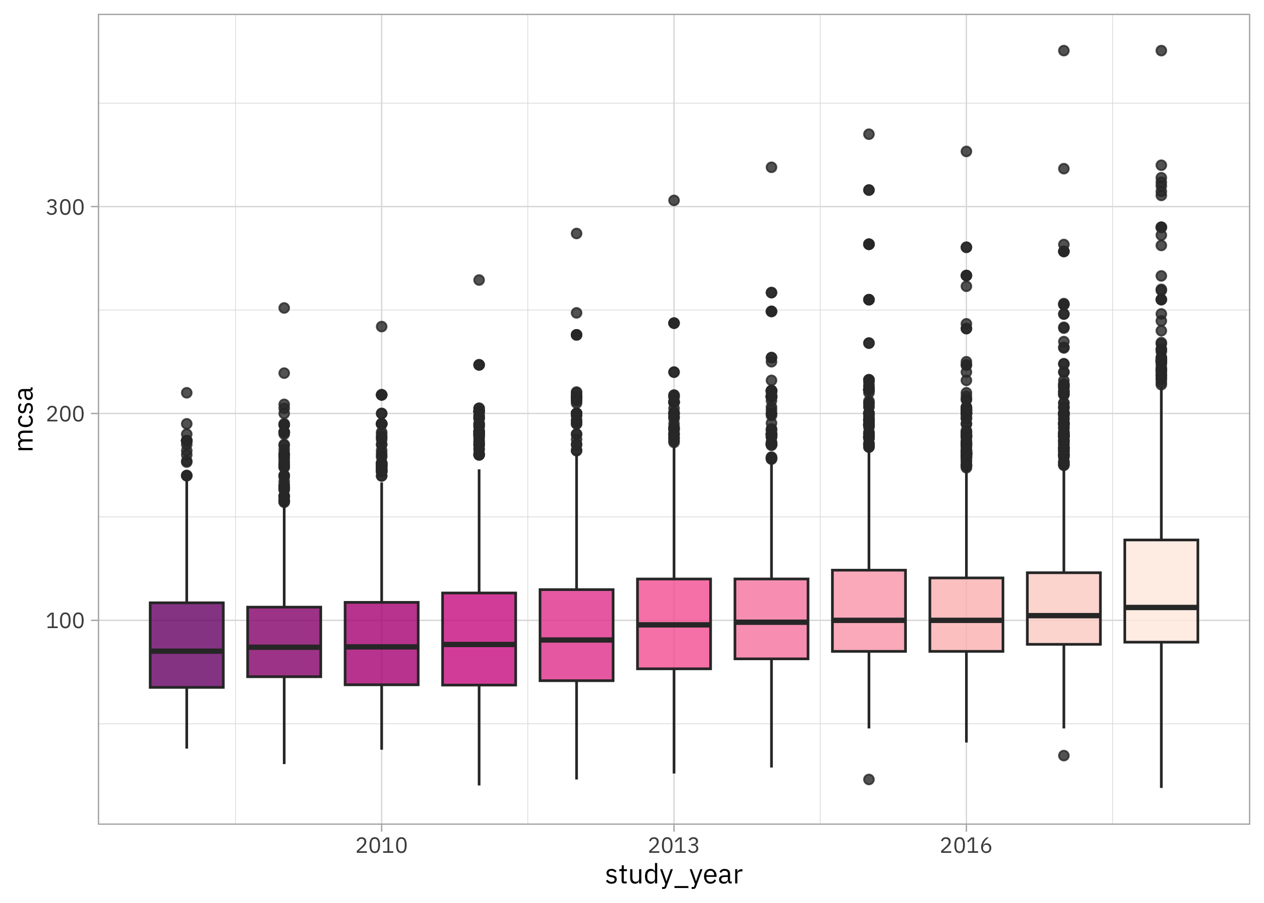
Before we get started with the modeling, let’s do a bit of exploratory data analysis. How have childcare costs as measured by mcsa (median weekly price for school-aged kids in childcare centers) changed over time?

childcare_costs |>
  ggplot(aes(study_year, mcsa, group = study_year, fill = study_year)) +
  geom_boxplot(alpha = 0.8, show.legend = FALSE) +
  scale_fill_distiller(palette = "RdPu")

How are childcare costs related to mhi_2018 (median household income) and flfpr_20to64 (labor force participation for women)?

childcare_costs |>
  ggplot(aes(mhi_2018, mcsa, color = flfpr_20to64)) +
  geom_point(alpha = 0.5) +
  scale_x_log10() +
  scale_color_viridis_c()

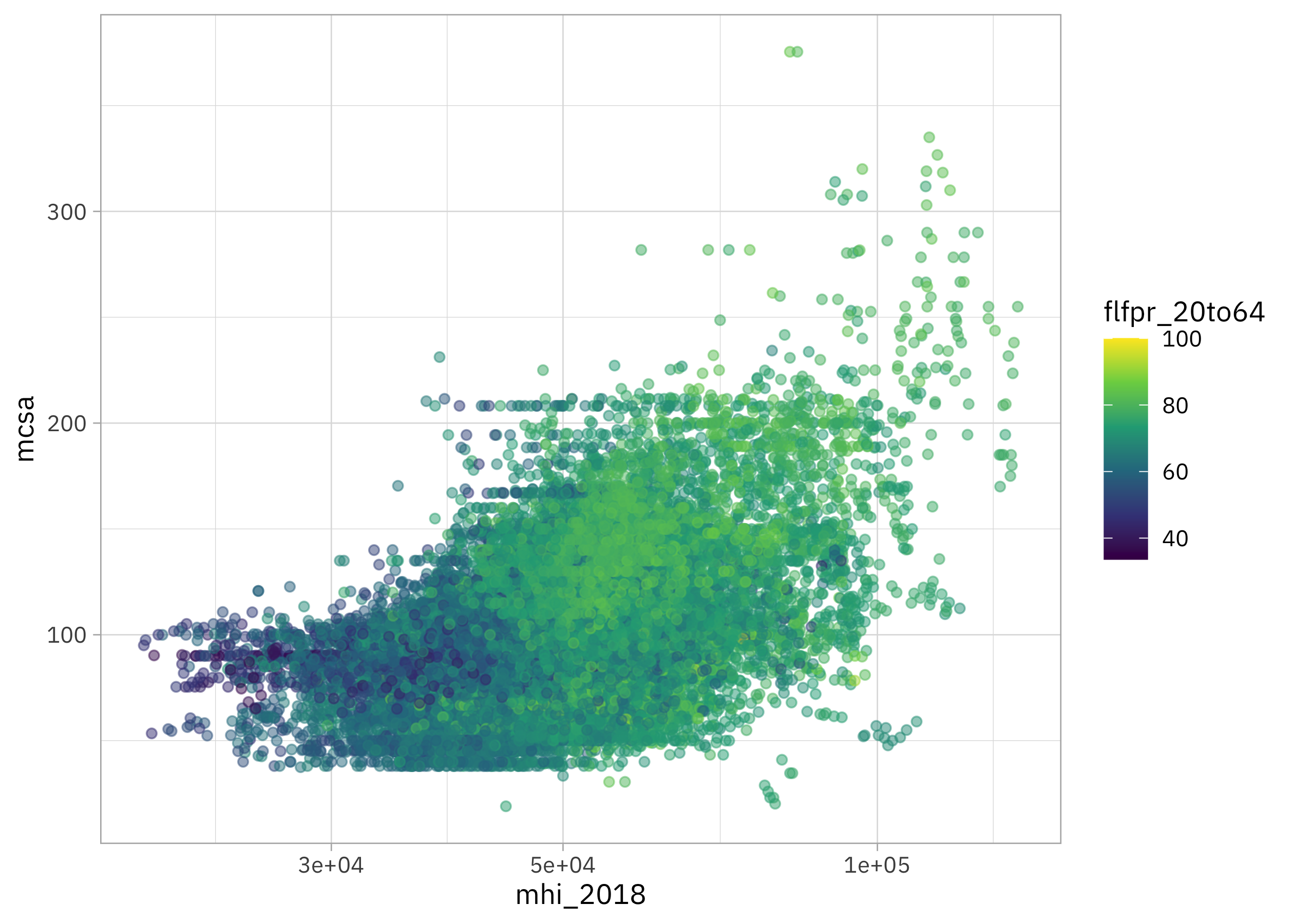
It looks like childcare costs are mostly flat for low income counties but increase for high income counties, and labor force participation for women is higher in high income counties.

What about the racial makeup of counties?

childcare_costs |>
  select(mcsa, starts_with("one_race"), mhi_2018) |>
  select(-one_race) |>
  pivot_longer(starts_with("one_race")) |>
  ggplot(aes(value, mcsa, color = mhi_2018)) +
  geom_point(alpha = 0.5) +
  facet_wrap(vars(name), scales = "free_x") +
  scale_color_viridis_c() +
  labs(x = "% of population")

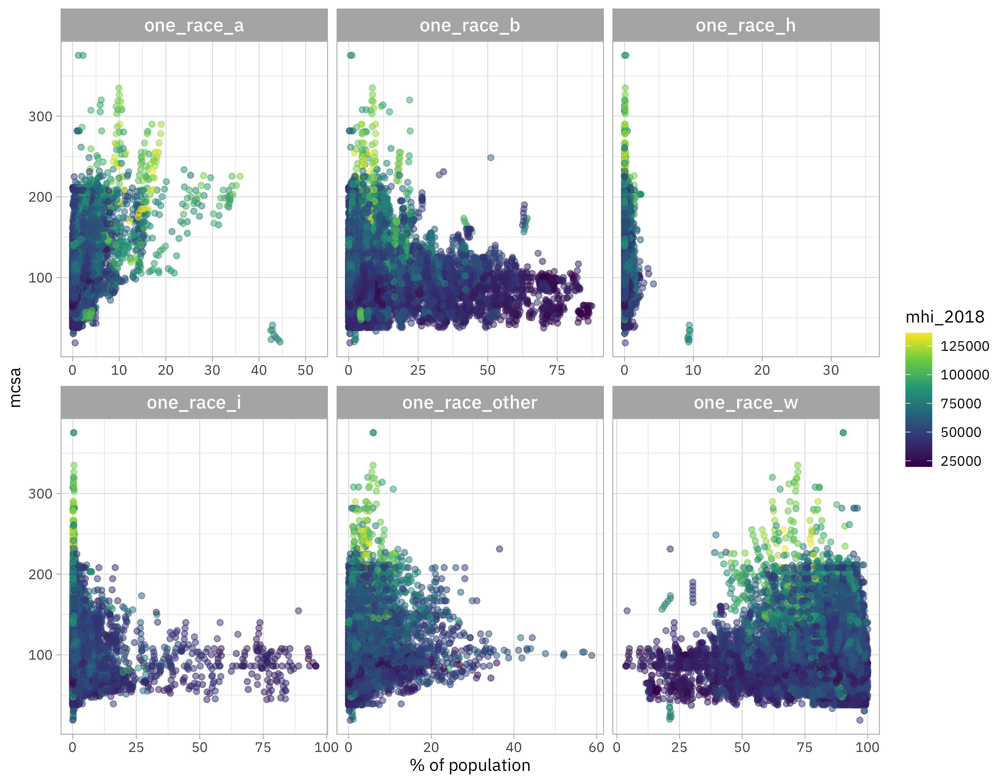
There’s a lot going on in this one! When a county has more Black population (one_race_b), household income is lower and childcare costs are lower; the opposite is true for the white population (one_race_w). There looks to be a trend for the Asian population (one_race_a) where a higher Asian population comes with higher childcare costs. None of these relationships are causal, of course, but related to complex relationships between race, class, and where people live in the US.

Build a model

Let’s start our modeling by setting up our “data budget.” For this example, let’s predict mcsa (costs for school-age kids in childcare centers) and remove the other measures of childcare costs for babies or toddlers, family-based childcare, etc. Let’s remove the FIPS codes which literally encode location and instead focus on the characteristics of counties like household income, number of households with children, and similar. Since this dataset is quite big, let’s use a single validation set.

library(tidymodels)

set.seed(123)
childcare_split <- childcare_costs |>
  select(-matches("^mc_|^mfc")) |>
  select(-county_fips_code) |>
  na.omit() |>
  initial_split(strata = mcsa)

childcare_train <- training(childcare_split)
childcare_test <- testing(childcare_split)

set.seed(234)
childcare_set <- validation_split(childcare_train)
childcare_set

## # Validation Set Split (0.75/0.25)
## # A tibble: 1 × 2
##   splits               id
##   <list>               <chr>
## 1 <split [13269/4424]> validation

All these predictors are already numeric so we don’t need any special feature engineering; we can just use a formula like mcsa ~ .. We do need to set up a tunable xgboost model specification with early stopping, like we planned. We will keep the number of trees as a constant (and not too terribly high), set stop_iter (the early stopping parameter) to tune(), and then tune a few other parameters. Notice that we need to set a validation set (which in this case is a proportion of the training set) to hold back to use for deciding when to stop.

xgb_spec <-
  boost_tree(
    trees = 500,
    min_n = tune(),
    mtry = tune(),
    stop_iter = tune(),
    learn_rate = 0.01
  ) |>
  set_engine("xgboost", validation = 0.2) |>
  set_mode("regression")

xgb_wf <- workflow(mcsa ~ ., xgb_spec)
xgb_wf

## ══ Workflow ════════════════════════════════════════════════════════════════════
## Preprocessor: Formula
## Model: boost_tree()
##
## ── Preprocessor ────────────────────────────────────────────────────────────────
## mcsa ~ .
##
## ── Model ───────────────────────────────────────────────────────────────────────
## Boosted Tree Model Specification (regression)
##
## Main Arguments:
##   mtry = tune()
##   trees = 500
##   min_n = tune()
##   learn_rate = 0.01
##   stop_iter = tune()
##
## Engine-Specific Arguments:
##   validation = 0.2
##
## Computational engine: xgboost

Our model is read to go! Let’s tune across possible hyperparameter configurations using our training set (with a subset that is held back for early stopping) plus our validation set.

doParallel::registerDoParallel()
set.seed(234)
xgb_rs <- tune_grid(xgb_wf, childcare_set, grid = 15)
xgb_rs

## # Tuning results
## # Validation Set Split (0.75/0.25)
## # A tibble: 1 × 4
##   splits               id         .metrics          .notes
##   <list>               <chr>      <list>            <list>
## 1 <split [13269/4424]> validation <tibble [30 × 7]> <tibble [0 × 3]>

All done!

Evaluate results

How did these results turn out? We can visualize them.

autoplot(xgb_rs)

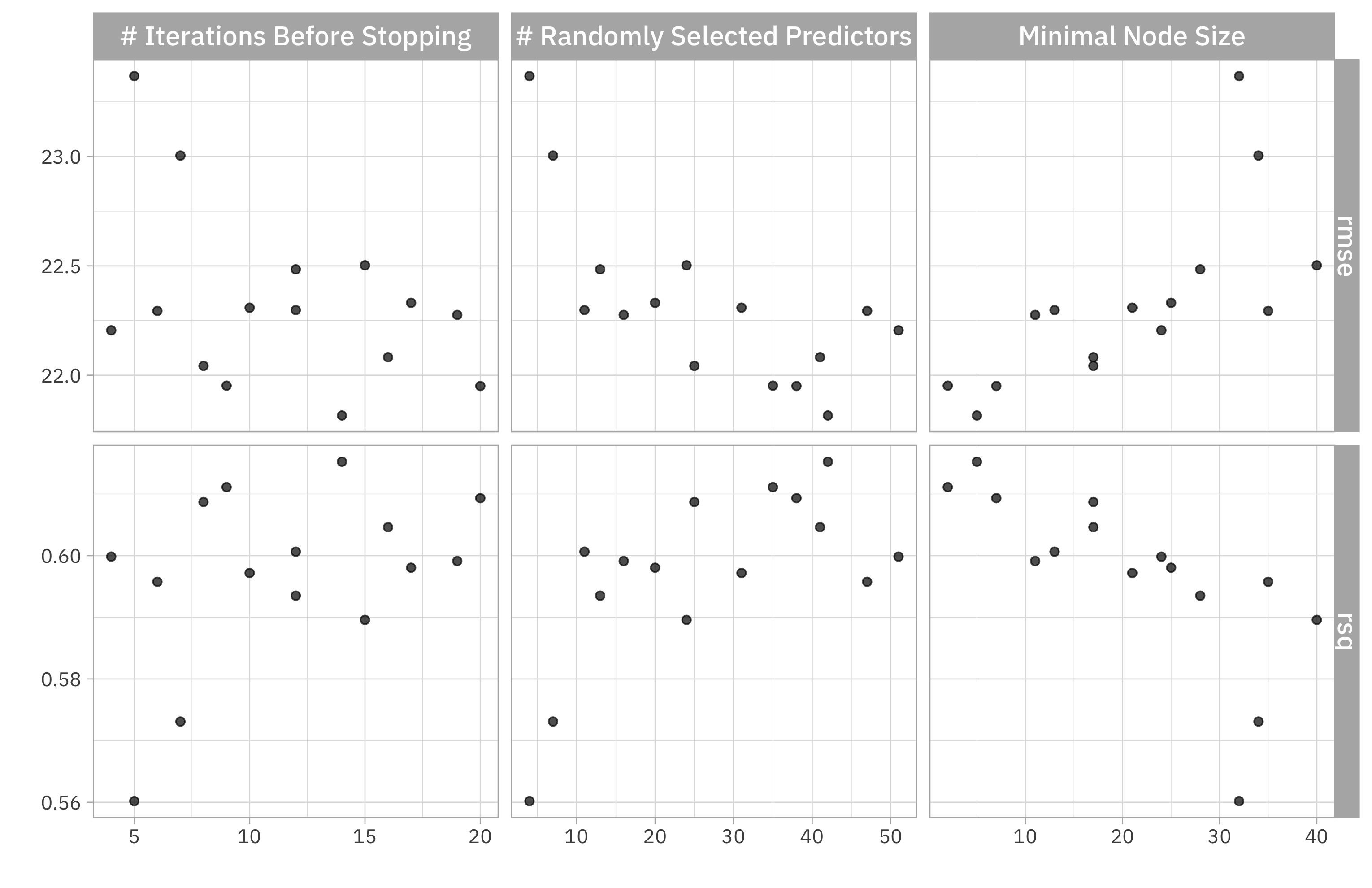
Maybe we could consider going back to tune again with lower min_n and/or higher mtry to achieve better performance.

We can look at the top results we got like this:

show_best(xgb_rs, "rmse")

## # A tibble: 5 × 9
##    mtry min_n stop_iter .metric .estimator  mean     n std_err .config
##   <int> <int>     <int> <chr>   <chr>      <dbl> <int>   <dbl> <chr>
## 1    42     5        14 rmse    standard    21.8     1      NA Preprocessor1_Mo…
## 2    38     7        20 rmse    standard    22.0     1      NA Preprocessor1_Mo…
## 3    35     2         9 rmse    standard    22.0     1      NA Preprocessor1_Mo…
## 4    25    17         8 rmse    standard    22.0     1      NA Preprocessor1_Mo…
## 5    41    17        16 rmse    standard    22.1     1      NA Preprocessor1_Mo…

The best RMSE is a little more than $20, which is an estimate of how precisely we can predict the median childcare cost in a US county (remember that the median in this dataset was about $100).

Let’s use last_fit() to fit one final time to the training data and evaluate one final time on the testing data, with the numerically optimal result from xgb_rs.

childcare_fit <- xgb_wf |>
  finalize_workflow(select_best(xgb_rs, "rmse")) |>
  last_fit(childcare_split)

childcare_fit

## # Resampling results
## # Manual resampling
## # A tibble: 1 × 6
##   splits               id              .metrics .notes   .predictions .workflow
##   <list>               <chr>           <list>   <list>   <list>       <list>
## 1 <split [17693/5900]> train/test spl… <tibble> <tibble> <tibble>     <workflow>

How did this model perform on the testing data, that was not used in tuning or training?

collect_metrics(childcare_fit)

## # A tibble: 2 × 4
##   .metric .estimator .estimate .config
##   <chr>   <chr>          <dbl> <chr>
## 1 rmse    standard      21.5   Preprocessor1_Model1
## 2 rsq     standard       0.625 Preprocessor1_Model1

What features are most important for this xgboost model?

library(vip)

extract_workflow(childcare_fit) |>
  extract_fit_parsnip() |>
  vip(num_features = 15, geom = "point")

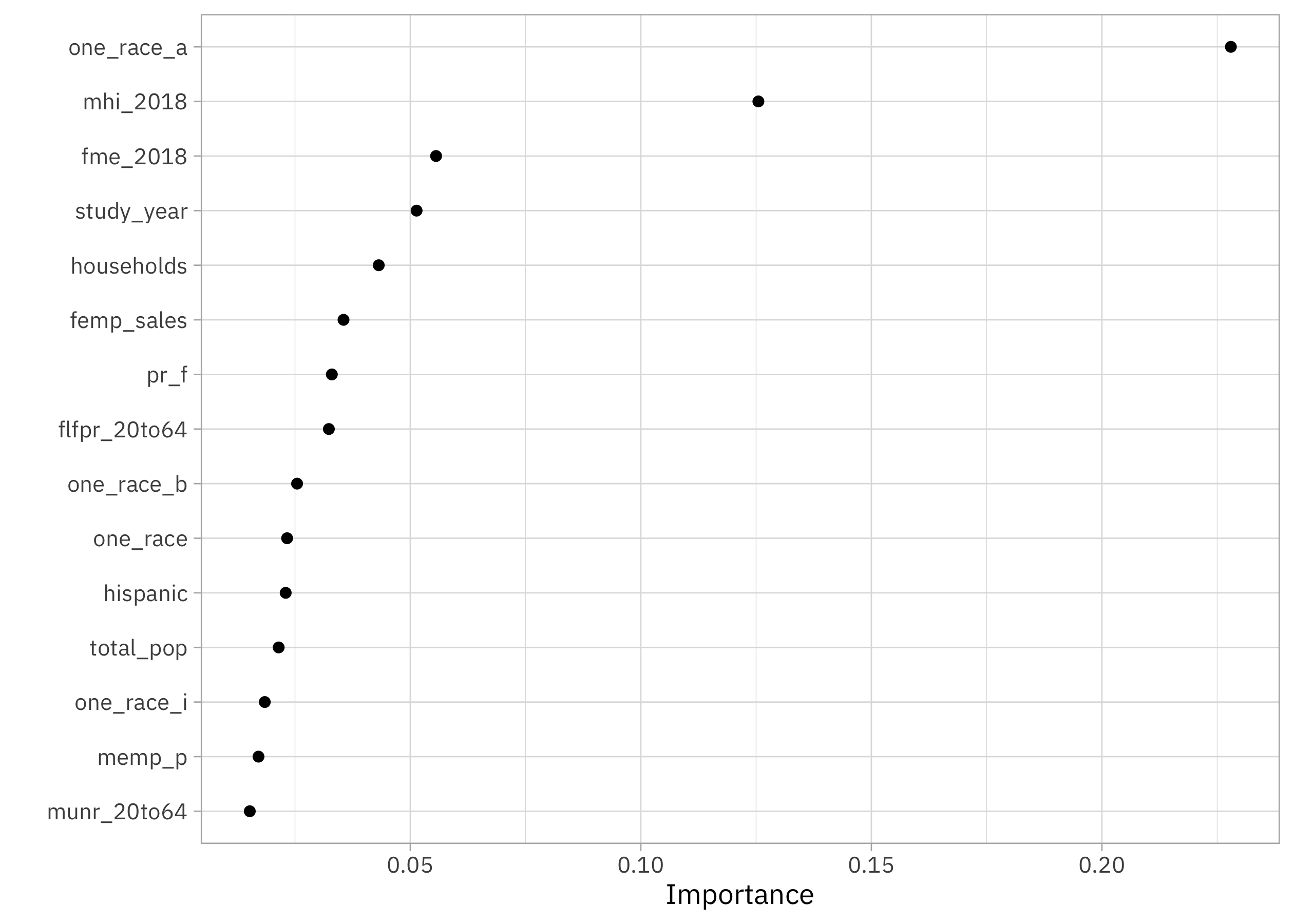
The proportion of county population that is Asian has a big impact in this model, as does median household income, median earnings for women, year, and number of households in the county.

BONUS: create a deployable model object!

If you wanted to deploy this model, the next step is to create a deployable model object with vetiver:

library(vetiver)
v <- extract_workflow(childcare_fit) |>
  vetiver_model("childcare-costs-xgb")
v

##
## ── childcare-costs-xgb ─ <bundled_workflow> model for deployment
## A xgboost regression modeling workflow using 52 features

At posit::conf() this coming September in Chicago, I am teaching a workshop on how to deploy and maintain models with vetiver. Registration is open now if you are interested in learning more about this part of the modeling process, but you should also check out all the other workshops being organized!