Text predictors for #TidyTuesday chocolate ratings

This is the latest in my series of screencasts demonstrating how to use the tidymodels packages, from just getting started to tuning more complex models. Today’s screencast is a good one for folks newer to tidymodels and focuses on predicting with text data, using this week’s #TidyTuesday dataset on chocolate ratings. 🍫

Here is the code I used in the video, for those who prefer reading instead of or in addition to video.

Explore data

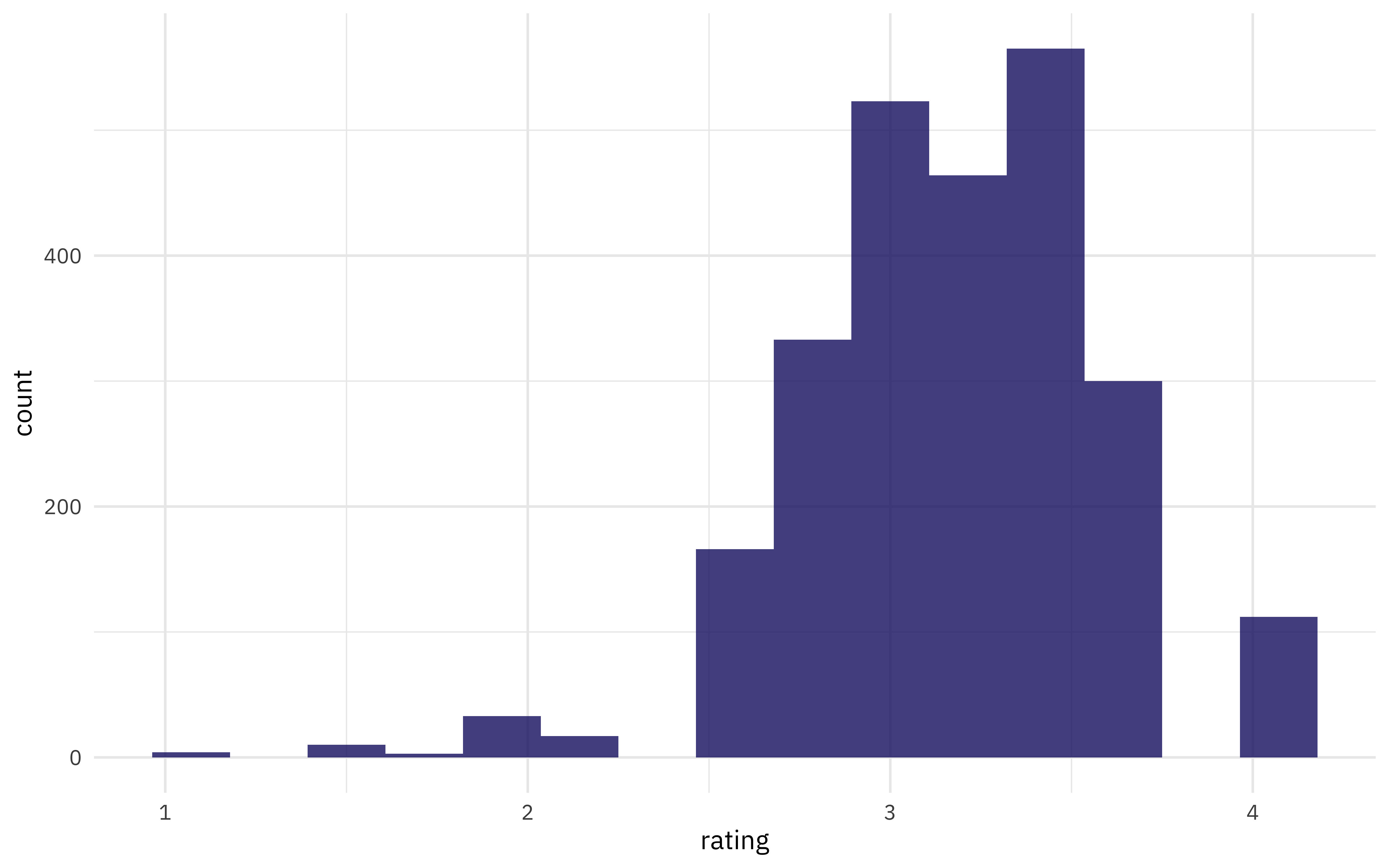
Our modeling goal is to predict ratings for chocolate based on the main characteristics as described by the raters. It’s not likely that we can build a high performing model using only these short text descriptions but we can use this dataset to demonstrate how to approach feature engineering for text. How are the ratings distributed?

library(tidyverse)

url <- "https://raw.githubusercontent.com/rfordatascience/tidytuesday/master/data/2022/2022-01-18/chocolate.csv"
chocolate <- read_csv(url)

chocolate %>%
  ggplot(aes(rating)) +
  geom_histogram(bins = 15)

What are the most common words used to describe the most memorable characteristics of each chocolate sample?

library(tidytext)

tidy_chocolate <-
  chocolate %>%
  unnest_tokens(word, most_memorable_characteristics)

tidy_chocolate %>%
  count(word, sort = TRUE)

## # A tibble: 547 × 2
##    word        n
##    <chr>   <int>
##  1 cocoa     419
##  2 sweet     318
##  3 nutty     278
##  4 fruit     273
##  5 roasty    228
##  6 mild      226
##  7 sour      208
##  8 earthy    199
##  9 creamy    189
## 10 intense   178
## # … with 537 more rows

What is the mean rating for these words?

tidy_chocolate %>%
  group_by(word) %>%
  summarise(
    n = n(),
    rating = mean(rating)
  ) %>%
  ggplot(aes(n, rating)) +
  geom_hline(
    yintercept = mean(chocolate$rating), lty = 2,
    color = "gray50", size = 1.5
  ) +
  geom_jitter(color = "midnightblue", alpha = 0.7) +
  geom_text(aes(label = word),
    check_overlap = TRUE, family = "IBMPlexSans",
    vjust = "top", hjust = "left"
  ) +
  scale_x_log10()

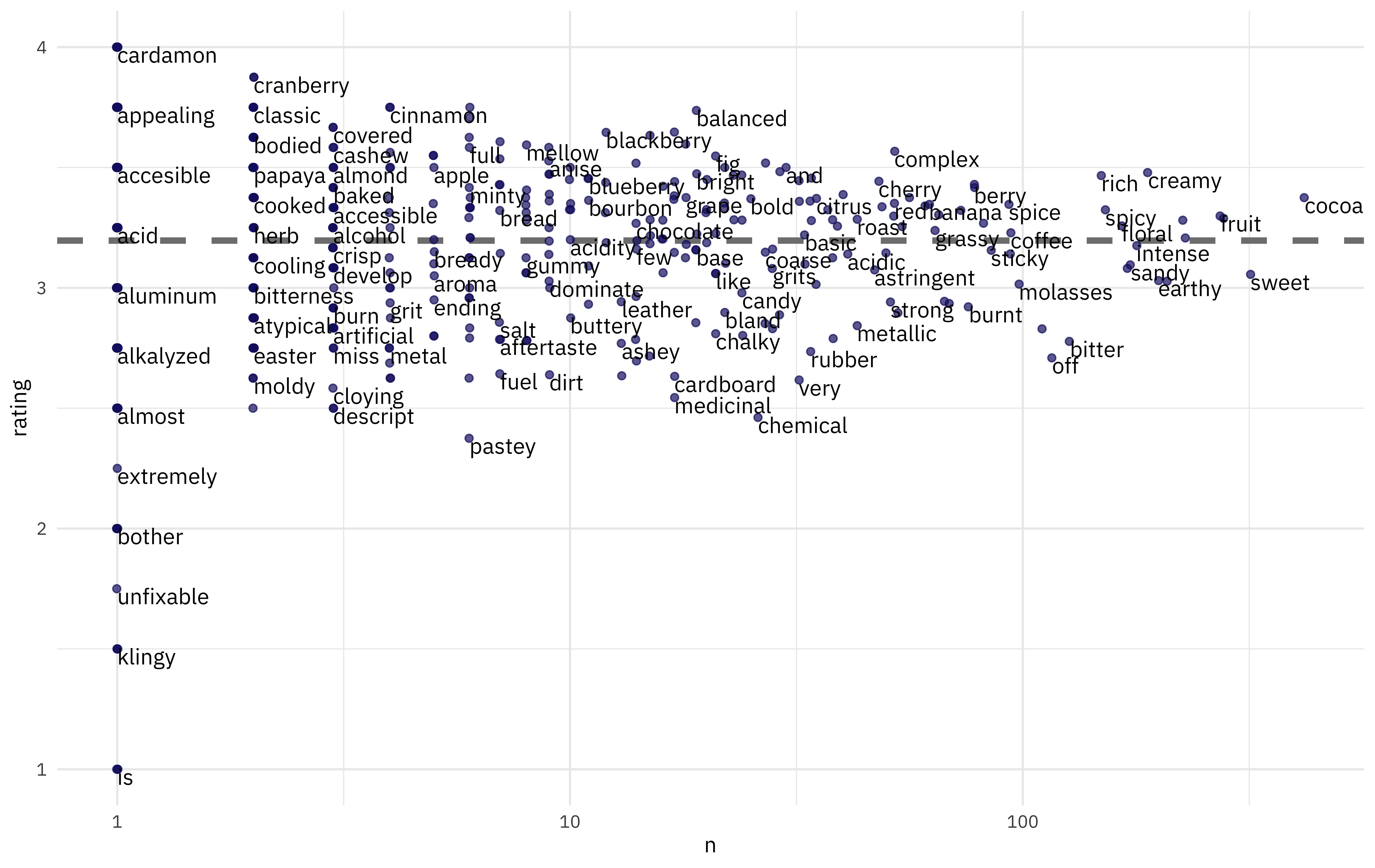
Complex, balanced chocolate is good, but burnt, pastey chocolate is bad.

Build models

Let’s start our modeling by setting up our “data budget.” We’ll stratify by our outcome rating.

library(tidymodels)

set.seed(123)
choco_split <- initial_split(chocolate, strata = rating)
choco_train <- training(choco_split)
choco_test <- testing(choco_split)

set.seed(234)
choco_folds <- vfold_cv(choco_train, strata = rating)
choco_folds

## #  10-fold cross-validation using stratification 
## # A tibble: 10 × 2
##    splits             id    
##    <list>             <chr> 
##  1 <split [1705/191]> Fold01
##  2 <split [1705/191]> Fold02
##  3 <split [1705/191]> Fold03
##  4 <split [1706/190]> Fold04
##  5 <split [1706/190]> Fold05
##  6 <split [1706/190]> Fold06
##  7 <split [1707/189]> Fold07
##  8 <split [1707/189]> Fold08
##  9 <split [1708/188]> Fold09
## 10 <split [1709/187]> Fold10

Next, let’s set up our feature engineering. We will need to transform our text data into features useful for our model by tokenizing and computing (in this case) tf-idf.

library(textrecipes)

choco_rec <-
  recipe(rating ~ most_memorable_characteristics, data = choco_train) %>%
  step_tokenize(most_memorable_characteristics) %>%
  step_tokenfilter(most_memorable_characteristics, max_tokens = 100) %>%
  step_tfidf(most_memorable_characteristics)

## just to check this works
prep(choco_rec) %>% bake(new_data = NULL)

## # A tibble: 1,896 × 101
##    rating tfidf_most_memor… tfidf_most_memor… tfidf_most_memor… tfidf_most_memo…
##     <dbl>             <dbl>             <dbl>             <dbl>            <dbl>
##  1   3                 0                    0                 0                0
##  2   2.75              0                    0                 0                0
##  3   3                 0                    0                 0                0
##  4   3                 0                    0                 0                0
##  5   2.75              0                    0                 0                0
##  6   3                 1.38                 0                 0                0
##  7   2.75              0                    0                 0                0
##  8   2.5               0                    0                 0                0
##  9   2.75              0                    0                 0                0
## 10   3                 0                    0                 0                0
## # … with 1,886 more rows, and 96 more variables:
## #   tfidf_most_memorable_characteristics_base <dbl>,
## #   tfidf_most_memorable_characteristics_basic <dbl>,
## #   tfidf_most_memorable_characteristics_berry <dbl>,
## #   tfidf_most_memorable_characteristics_bitter <dbl>,
## #   tfidf_most_memorable_characteristics_black <dbl>,
## #   tfidf_most_memorable_characteristics_bland <dbl>, …

Now let’s create two model specifications to compare. Random forests are not known for performing well with natural language predictors, but this dataset involves very short text descriptions so let’s give it a try. Support vector machines do tend to work well with text data so let’s include that one too.

rf_spec <-
  rand_forest(trees = 500) %>%
  set_mode("regression")

rf_spec

## Random Forest Model Specification (regression)
## 
## Main Arguments:
##   trees = 500
## 
## Computational engine: ranger

svm_spec <-
  svm_linear() %>%
  set_mode("regression")

svm_spec

## Linear Support Vector Machine Specification (regression)
## 
## Computational engine: LiblineaR

Now it’s time to put the preprocessing and model together in a workflow(). The SVM requires the predictors to all be on the same scale, but all our predictors are now tf-idf values so we should be pretty much fine.

svm_wf <- workflow(choco_rec, svm_spec)
rf_wf <- workflow(choco_rec, rf_spec)

Evaluate models

These workflows have no tuning parameters so we can evaluate them as they are. (Random forest models can be tuned but they tend to work fine with the defaults as long as you have enough trees.)

doParallel::registerDoParallel()
contrl_preds <- control_resamples(save_pred = TRUE)

svm_rs <- fit_resamples(
  svm_wf,
  resamples = choco_folds,
  control = contrl_preds
)

ranger_rs <- fit_resamples(
  rf_wf,
  resamples = choco_folds,
  control = contrl_preds
)

How did these two models compare?

collect_metrics(svm_rs)

## # A tibble: 2 × 6
##   .metric .estimator  mean     n std_err .config             
##   <chr>   <chr>      <dbl> <int>   <dbl> <chr>               
## 1 rmse    standard   0.349    10 0.00627 Preprocessor1_Model1
## 2 rsq     standard   0.365    10 0.0175  Preprocessor1_Model1

collect_metrics(ranger_rs)

## # A tibble: 2 × 6
##   .metric .estimator  mean     n std_err .config             
##   <chr>   <chr>      <dbl> <int>   <dbl> <chr>               
## 1 rmse    standard   0.351    10 0.00714 Preprocessor1_Model1
## 2 rsq     standard   0.356    10 0.0163  Preprocessor1_Model1

We can visualize these results by comparing the predicted rating with the true rating:

bind_rows(
  collect_predictions(svm_rs) %>%
    mutate(mod = "SVM"),
  collect_predictions(ranger_rs) %>%
    mutate(mod = "ranger")
) %>%
  ggplot(aes(rating, .pred, color = id)) +
  geom_abline(lty = 2, color = "gray50", size = 1.2) +
  geom_jitter(width = 0.5, alpha = 0.5) +
  facet_wrap(vars(mod)) +
  coord_fixed()

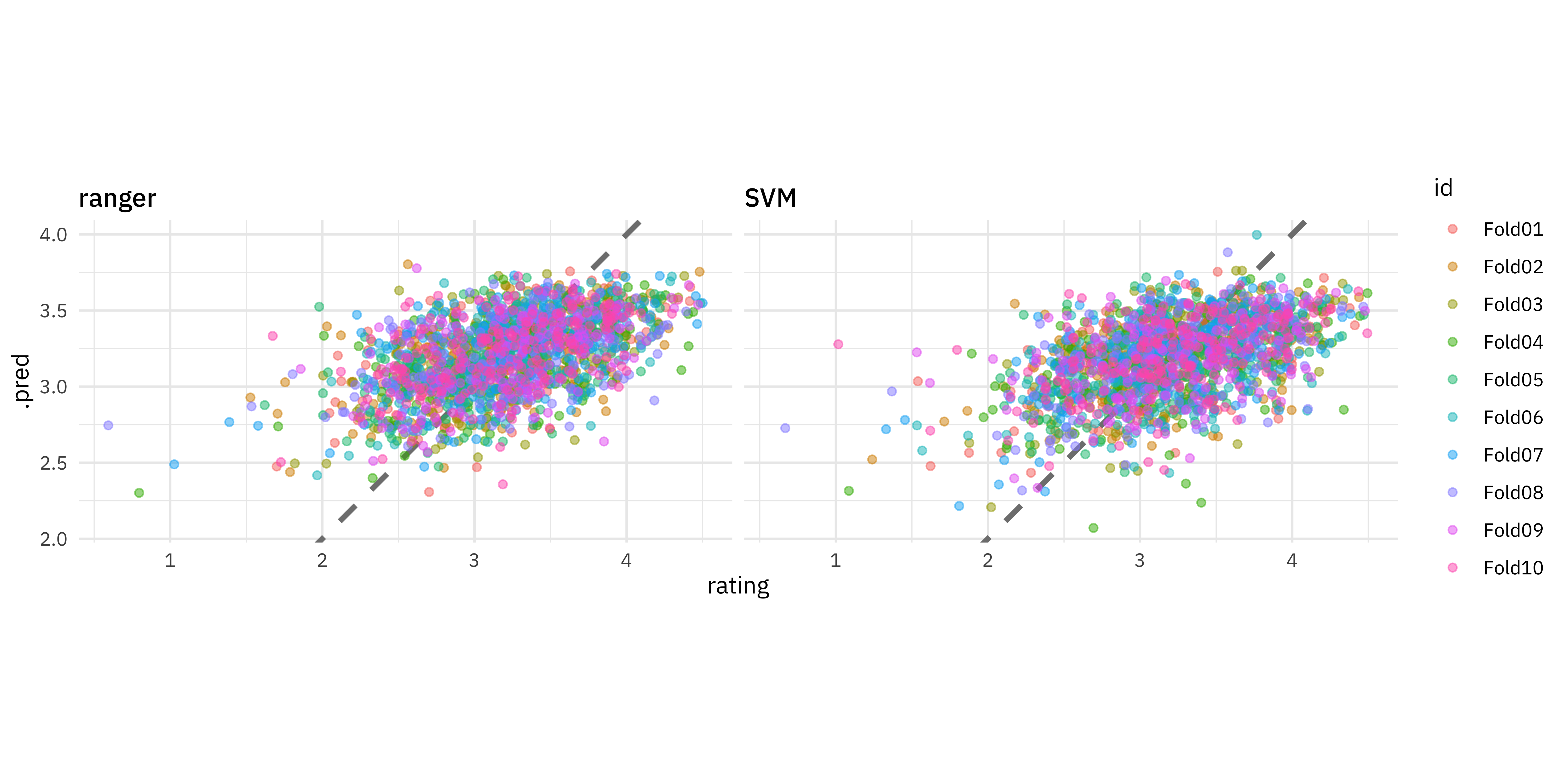
These models are not great but they perform pretty similarly, so perhaps we would choose the faster-to-train, linear SVM model. The function last_fit() fits one final time on the training data and evaluates on the testing data. This is the first time we have used the testing data.

final_fitted <- last_fit(svm_wf, choco_split)
collect_metrics(final_fitted) ## metrics evaluated on the *testing* data

## # A tibble: 2 × 4
##   .metric .estimator .estimate .config             
##   <chr>   <chr>          <dbl> <chr>               
## 1 rmse    standard       0.380 Preprocessor1_Model1
## 2 rsq     standard       0.348 Preprocessor1_Model1

This object contains a fitted workflow that we can use for prediction.

final_wf <- extract_workflow(final_fitted)
predict(final_wf, choco_test[55, ])

## # A tibble: 1 × 1
##   .pred
##   <dbl>
## 1  3.00

You can save this fitted final_wf object to use later with new data, for example with readr::write_rds().

One nice aspect of using a linear model is that we can directly inspect the coefficients for each term. Which words are more associated with high ratings vs. low ratings?

extract_workflow(final_fitted) %>%
  tidy() %>%
  filter(term != "Bias") %>%
  group_by(estimate > 0) %>%
  slice_max(abs(estimate), n = 10) %>%
  ungroup() %>%
  mutate(term = str_remove(term, "tfidf_most_memorable_characteristics_")) %>%
  ggplot(aes(estimate, fct_reorder(term, estimate), fill = estimate > 0)) +
  geom_col(alpha = 0.8) +
  scale_fill_discrete(labels = c("low ratings", "high ratings")) +
  labs(y = NULL, fill = "More from...")

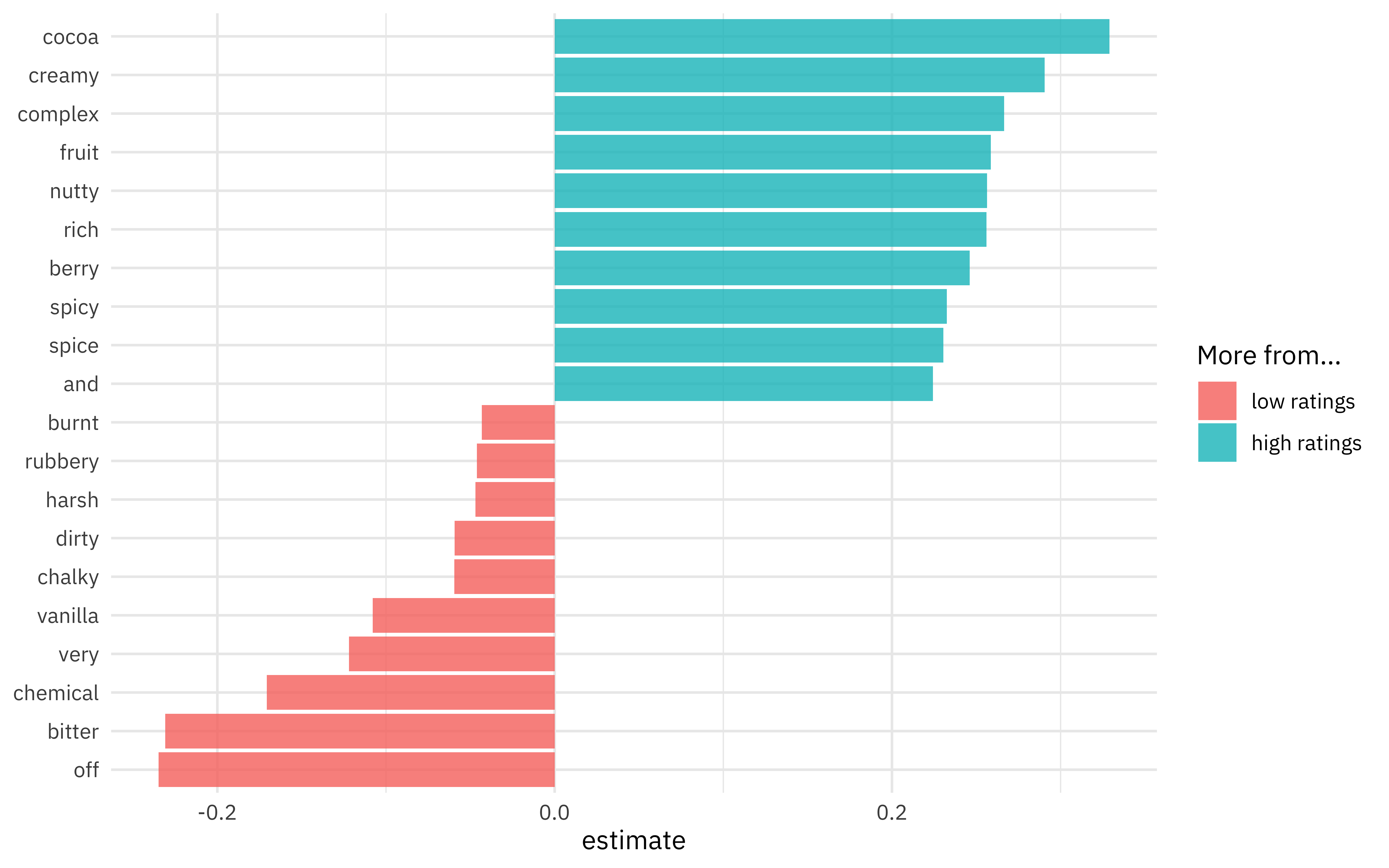
I know I personally would prefer creamy, rich chocolate to bitter, chalky chocolate!