Predict ratings for #TidyTuesday board games

This is the latest in my series of screencasts demonstrating how to use the tidymodels packages, from just getting started to tuning more complex models. That is the topic of today’s more advanced screencast, using this week’s #TidyTuesday dataset on board games. 🎲

Here is the code I used in the video, for those who prefer reading instead of or in addition to video.

Explore data

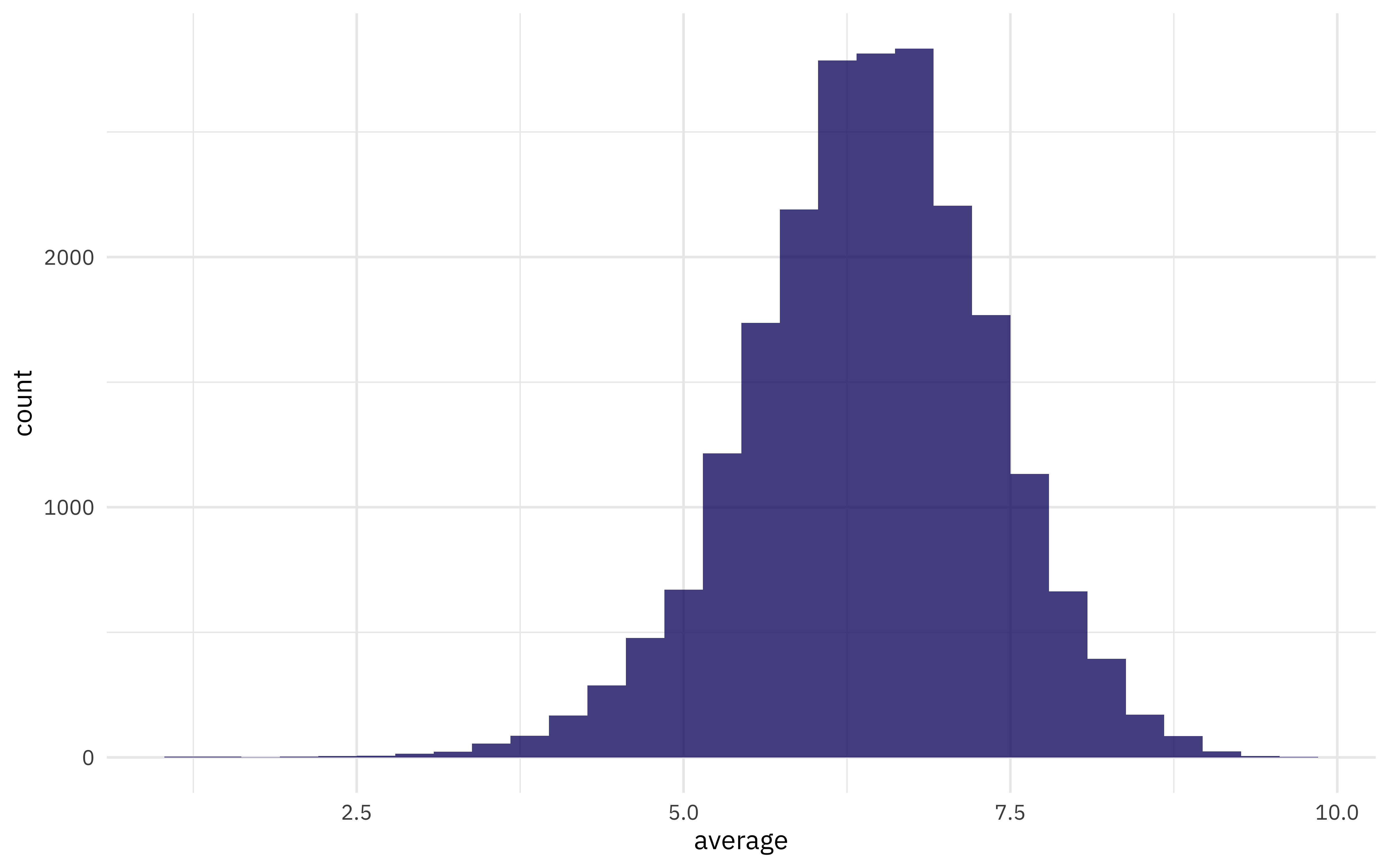
Our modeling goal is to predict ratings for board games based on the main characteristics like number of players and game category. How are the ratings distributed?

library(tidyverse)

ratings <- read_csv("https://raw.githubusercontent.com/rfordatascience/tidytuesday/master/data/2022/2022-01-25/ratings.csv")
details <- read_csv("https://raw.githubusercontent.com/rfordatascience/tidytuesday/master/data/2022/2022-01-25/details.csv")

ratings_joined <-
  ratings %>%
  left_join(details, by = "id")

ggplot(ratings_joined, aes(average)) +
  geom_histogram(alpha = 0.8)

This is a pretty sizeable rectangular dataset so let’s use an xgboost model; xgboost is a good fit for that type of dataset. How is a characteristic like the minimum recommended age for the game related to the rating?

ratings_joined %>%
  filter(!is.na(minage)) %>%
  mutate(minage = cut_number(minage, 4)) %>%
  ggplot(aes(minage, average, fill = minage)) +
  geom_boxplot(alpha = 0.2, show.legend = FALSE)

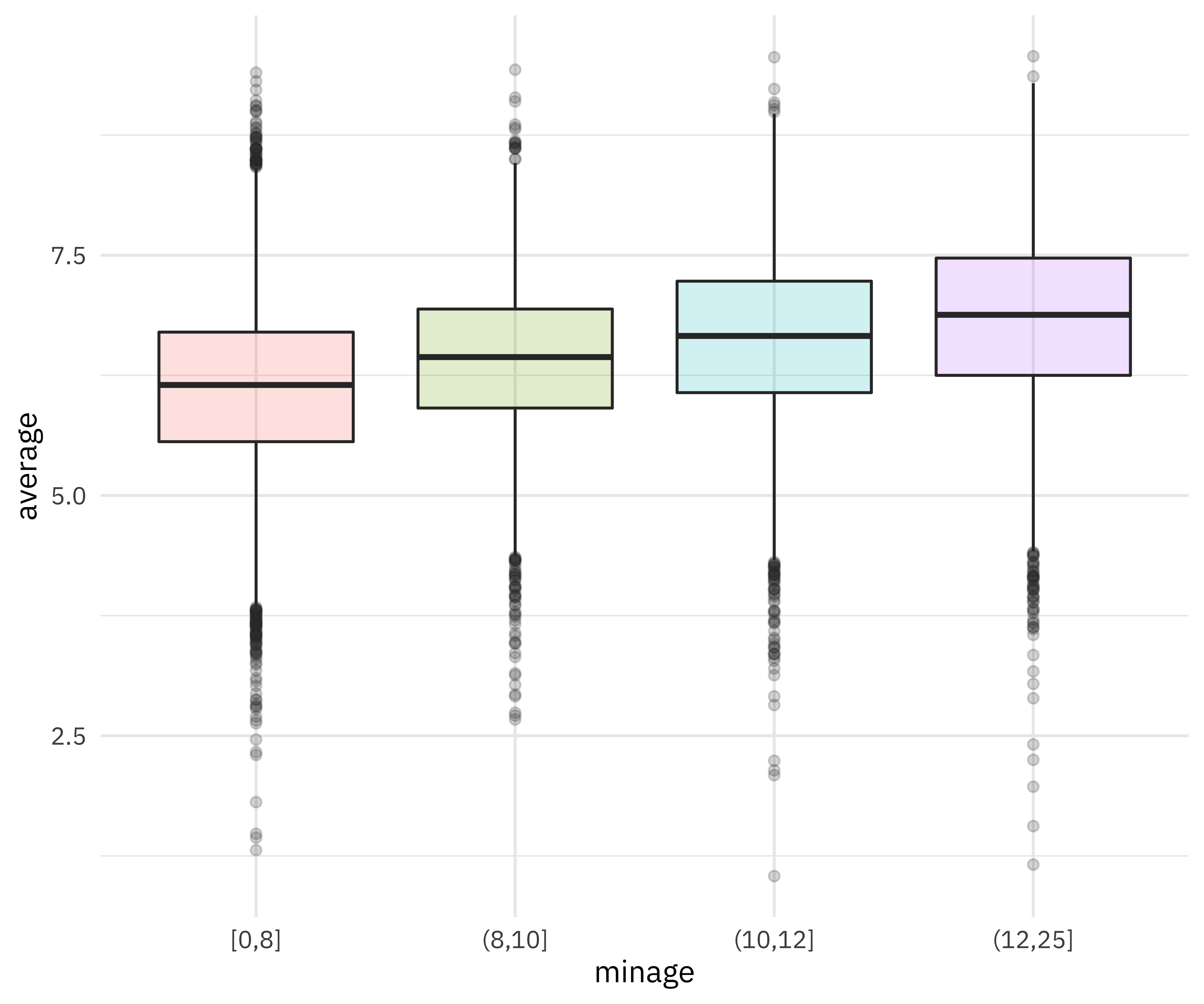
This kind of relationship is what we hope our xgboost model can use.

Tune an xgboost model

Let’s start our modeling by setting up our “data budget.” We’ll subset down to only variables like minimum/maximum age and playing time, and stratify by our outcome average.

library(tidymodels)

set.seed(123)
game_split <-
  ratings_joined %>%
  select(name, average, matches("min|max"), boardgamecategory) %>%
  na.omit() %>%
  initial_split(strata = average)
game_train <- training(game_split)
game_test <- testing(game_split)

set.seed(234)
game_folds <- vfold_cv(game_train, strata = average)
game_folds

## #  10-fold cross-validation using stratification 
## # A tibble: 10 × 2
##    splits               id    
##    <list>               <chr> 
##  1 <split [14407/1602]> Fold01
##  2 <split [14407/1602]> Fold02
##  3 <split [14407/1602]> Fold03
##  4 <split [14408/1601]> Fold04
##  5 <split [14408/1601]> Fold05
##  6 <split [14408/1601]> Fold06
##  7 <split [14408/1601]> Fold07
##  8 <split [14408/1601]> Fold08
##  9 <split [14410/1599]> Fold09
## 10 <split [14410/1599]> Fold10

Next, let’s set up our feature engineering. In the screencast, I walk through starting with default tokenizing and then creating a custom tokenizer. Sometimes a dataset requires more care and custom feature engineering; the tidymodels ecosystem provides lots of fluent options for common use cases and then the ability to extend our framework for more specific needs while maintaining good statistical practice.

library(textrecipes)

split_category <- function(x) {
  x %>%
    str_split(", ") %>%
    map(str_remove_all, "[:punct:]") %>%
    map(str_squish) %>%
    map(str_to_lower) %>%
    map(str_replace_all, " ", "_")
}

game_rec <-
  recipe(average ~ ., data = game_train) %>%
  update_role(name, new_role = "id") %>%
  step_tokenize(boardgamecategory, custom_token = split_category) %>%
  step_tokenfilter(boardgamecategory, max_tokens = 30) %>%
  step_tf(boardgamecategory)

## just to make sure this works as expected
game_prep <- prep(game_rec)
bake(game_prep, new_data = NULL) %>% str()

## tibble [16,009 × 37] (S3: tbl_df/tbl/data.frame)
##  $ name                                      : Factor w/ 15781 levels "¡Adiós Calavera!",..: 10857 8587 14642 858 15729 6819 13313 1490 3143 9933 ...
##  $ minplayers                                : num [1:16009] 2 2 2 4 2 1 2 2 4 2 ...
##  $ maxplayers                                : num [1:16009] 6 8 10 10 6 8 6 2 16 6 ...
##  $ minplaytime                               : num [1:16009] 120 60 30 30 60 20 60 30 60 45 ...
##  $ maxplaytime                               : num [1:16009] 120 180 30 30 90 20 60 30 60 45 ...
##  $ minage                                    : num [1:16009] 10 8 6 12 15 6 8 8 13 8 ...
##  $ average                                   : num [1:16009] 5.59 4.37 5.41 5.79 5.8 5.62 4.31 4.66 5.68 5.14 ...
##  $ tf_boardgamecategory_abstract_strategy    : num [1:16009] 0 0 0 0 0 0 0 0 0 0 ...
##  $ tf_boardgamecategory_action_dexterity     : num [1:16009] 0 0 0 0 0 1 0 0 0 0 ...
##  $ tf_boardgamecategory_adventure            : num [1:16009] 0 0 0 0 0 0 0 0 0 0 ...
##  $ tf_boardgamecategory_ancient              : num [1:16009] 0 0 0 0 0 0 0 0 0 0 ...
##  $ tf_boardgamecategory_animals              : num [1:16009] 0 0 0 0 0 0 0 0 0 0 ...
##  $ tf_boardgamecategory_bluffing             : num [1:16009] 0 0 0 0 0 0 0 0 0 0 ...
##  $ tf_boardgamecategory_card_game            : num [1:16009] 0 0 1 1 0 0 0 0 0 1 ...
##  $ tf_boardgamecategory_childrens_game       : num [1:16009] 0 0 0 0 0 0 1 1 0 0 ...
##  $ tf_boardgamecategory_deduction            : num [1:16009] 0 0 0 0 0 0 0 1 0 0 ...
##  $ tf_boardgamecategory_dice                 : num [1:16009] 0 0 0 0 0 0 0 0 0 0 ...
##  $ tf_boardgamecategory_economic             : num [1:16009] 0 1 0 0 0 0 1 0 0 0 ...
##  $ tf_boardgamecategory_exploration          : num [1:16009] 0 0 0 0 1 0 0 0 0 0 ...
##  $ tf_boardgamecategory_fantasy              : num [1:16009] 0 0 0 0 0 0 0 0 0 0 ...
##  $ tf_boardgamecategory_fighting             : num [1:16009] 0 0 0 0 1 0 0 0 0 0 ...
##  $ tf_boardgamecategory_horror               : num [1:16009] 0 0 0 0 1 0 0 0 0 0 ...
##  $ tf_boardgamecategory_humor                : num [1:16009] 0 0 0 1 0 0 0 0 0 0 ...
##  $ tf_boardgamecategory_medieval             : num [1:16009] 0 0 0 0 0 0 0 0 0 0 ...
##  $ tf_boardgamecategory_miniatures           : num [1:16009] 0 0 0 0 1 0 0 0 0 0 ...
##  $ tf_boardgamecategory_movies_tv_radio_theme: num [1:16009] 0 0 1 0 1 0 0 0 0 0 ...
##  $ tf_boardgamecategory_nautical             : num [1:16009] 0 0 0 0 0 0 0 1 0 0 ...
##  $ tf_boardgamecategory_negotiation          : num [1:16009] 0 1 0 0 0 0 0 0 0 0 ...
##  $ tf_boardgamecategory_party_game           : num [1:16009] 0 0 0 1 0 1 0 0 1 0 ...
##  $ tf_boardgamecategory_print_play           : num [1:16009] 0 0 0 0 0 0 0 0 0 0 ...
##  $ tf_boardgamecategory_puzzle               : num [1:16009] 0 0 0 0 0 0 0 0 1 0 ...
##  $ tf_boardgamecategory_racing               : num [1:16009] 0 0 0 0 0 0 0 0 0 0 ...
##  $ tf_boardgamecategory_realtime             : num [1:16009] 0 0 0 0 0 0 0 0 0 0 ...
##  $ tf_boardgamecategory_science_fiction      : num [1:16009] 0 0 0 0 0 0 0 0 0 0 ...
##  $ tf_boardgamecategory_trivia               : num [1:16009] 0 0 0 0 0 0 0 0 1 0 ...
##  $ tf_boardgamecategory_wargame              : num [1:16009] 1 0 0 0 0 0 0 1 0 0 ...
##  $ tf_boardgamecategory_world_war_ii         : num [1:16009] 0 0 0 0 0 0 0 0 0 0 ...

Now let’s create a tunable xgboost model specification, with only some of the most important hyperparameters tunable, and combine it with our preprocessing recipe in a workflow(). To achieve higher performance, we could try more careful and/or extensive choices for hyperparameter tuning.

xgb_spec <-
  boost_tree(
    trees = tune(),
    mtry = tune(),
    min_n = tune(),
    learn_rate = 0.01
  ) %>%
  set_engine("xgboost") %>%
  set_mode("regression")

xgb_wf <- workflow(game_rec, xgb_spec)
xgb_wf

## ══ Workflow ════════════════════════════════════════════════════════════════════
## Preprocessor: Recipe
## Model: boost_tree()
## 
## ── Preprocessor ────────────────────────────────────────────────────────────────
## 3 Recipe Steps
## 
## • step_tokenize()
## • step_tokenfilter()
## • step_tf()
## 
## ── Model ───────────────────────────────────────────────────────────────────────
## Boosted Tree Model Specification (regression)
## 
## Main Arguments:
##   mtry = tune()
##   trees = tune()
##   min_n = tune()
##   learn_rate = 0.01
## 
## Computational engine: xgboost

Now we can use tune_race_anova() to eliminate parameter combinations that are not doing well.

library(finetune)
doParallel::registerDoParallel()

set.seed(234)
xgb_game_rs <-
  tune_race_anova(
    xgb_wf,
    game_folds,
    grid = 20,
    control = control_race(verbose_elim = TRUE)
  )

xgb_game_rs

## # Tuning results
## # 10-fold cross-validation using stratification 
## # A tibble: 10 × 5
##    splits               id     .order .metrics          .notes          
##    <list>               <chr>   <int> <list>            <list>          
##  1 <split [14407/1602]> Fold03      1 <tibble [40 × 7]> <tibble [0 × 1]>
##  2 <split [14408/1601]> Fold05      2 <tibble [40 × 7]> <tibble [0 × 1]>
##  3 <split [14410/1599]> Fold10      3 <tibble [40 × 7]> <tibble [0 × 1]>
##  4 <split [14408/1601]> Fold06      4 <tibble [28 × 7]> <tibble [0 × 1]>
##  5 <split [14408/1601]> Fold08      5 <tibble [14 × 7]> <tibble [0 × 1]>
##  6 <split [14407/1602]> Fold01      6 <tibble [12 × 7]> <tibble [0 × 1]>
##  7 <split [14408/1601]> Fold04      7 <tibble [10 × 7]> <tibble [0 × 1]>
##  8 <split [14407/1602]> Fold02      8 <tibble [6 × 7]>  <tibble [0 × 1]>
##  9 <split [14410/1599]> Fold09      9 <tibble [6 × 7]>  <tibble [0 × 1]>
## 10 <split [14408/1601]> Fold07     10 <tibble [6 × 7]>  <tibble [0 × 1]>

Done!

Evaluate models

We can visualize how the possible parameter combinations we tried did during the “race.” Notice how we saved a TON of time by not evaluating the parameter combinations that were clearly doing poorly on all the resamples; we only kept going with the good parameter combinations.

plot_race(xgb_game_rs)

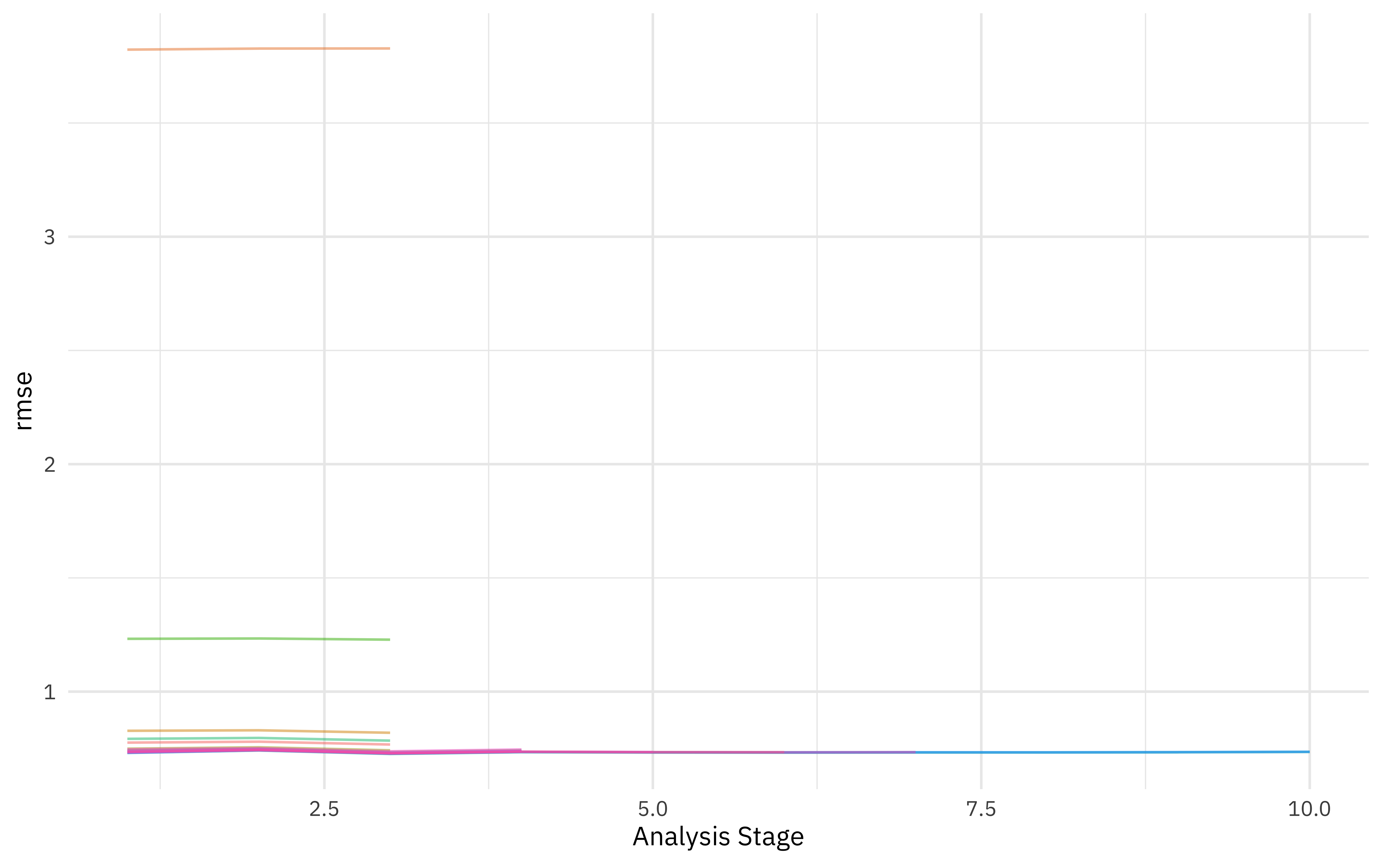
We ended up with three hyperparameter configurations in the end, all of which are pretty much the same.

show_best(xgb_game_rs)

## # A tibble: 3 × 9
##    mtry trees min_n .metric .estimator  mean     n std_err .config              
##   <int> <int> <int> <chr>   <chr>      <dbl> <int>   <dbl> <chr>                
## 1    14  1709    17 rmse    standard   0.735    10 0.00548 Preprocessor1_Model08
## 2    23  1652    29 rmse    standard   0.735    10 0.00526 Preprocessor1_Model13
## 3    25  1941    22 rmse    standard   0.735    10 0.00539 Preprocessor1_Model14

Let’s use last_fit() to fit one final time to the training data and evaluate one final time on the testing data.

xgb_last <-
  xgb_wf %>%
  finalize_workflow(select_best(xgb_game_rs, "rmse")) %>%
  last_fit(game_split)

xgb_last

## # Resampling results
## # Manual resampling 
## # A tibble: 1 × 6
##   splits               id              .metrics .notes   .predictions .workflow 
##   <list>               <chr>           <list>   <list>   <list>       <list>    
## 1 <split [16009/5339]> train/test spl… <tibble> <tibble> <tibble>     <workflow>

An xgboost model is not directly interpretable but we have several options for understanding why the model makes the predictions it does. Check out Chapter 18 of Tidy Modeling with R for more on model interpretability with tidymodels.

Let’s start with model-based variable importance using the vip package.

library(vip)

xgb_fit <- extract_fit_parsnip(xgb_last)
vip(xgb_fit, geom = "point", num_features = 12)

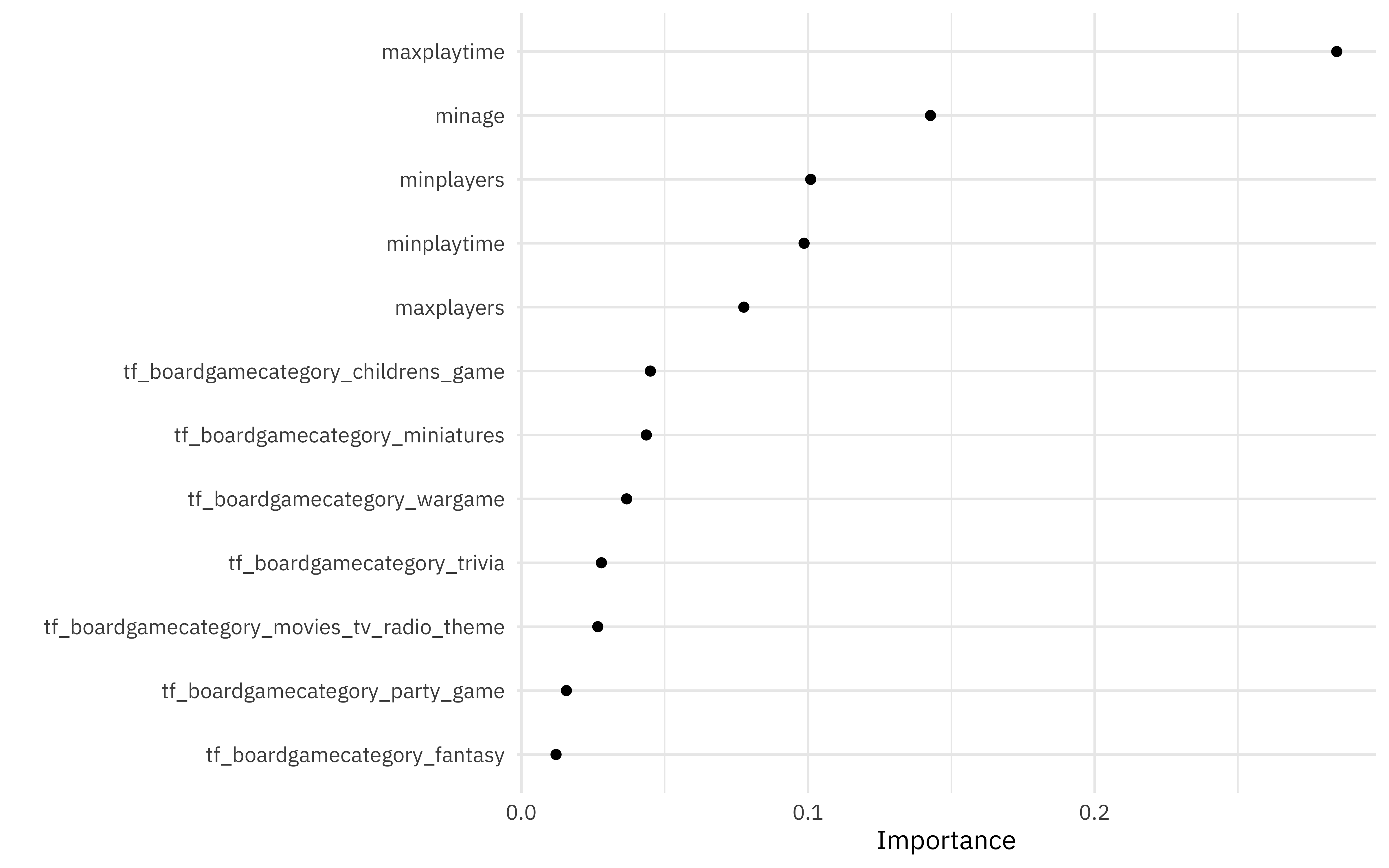
The maximum playing time and minimum age are the most important predictors driving the predicted game rating.

We can also use a model-agnostic approach like Shapley Additive Explanations, where the average contributions of features are computed under different combinations or “coalitions” of feature orderings. The SHAPforxgboost package makes setting this up for an xgboost model particularly nice.

We start by computing what we need for SHAP values, with the underlying xgboost engine fit and the predictors in a matrix format.

library(SHAPforxgboost)

game_shap <-
  shap.prep(
    xgb_model = extract_fit_engine(xgb_fit),
    X_train = bake(game_prep,
      has_role("predictor"),
      new_data = NULL,
      composition = "matrix"
    )
  )

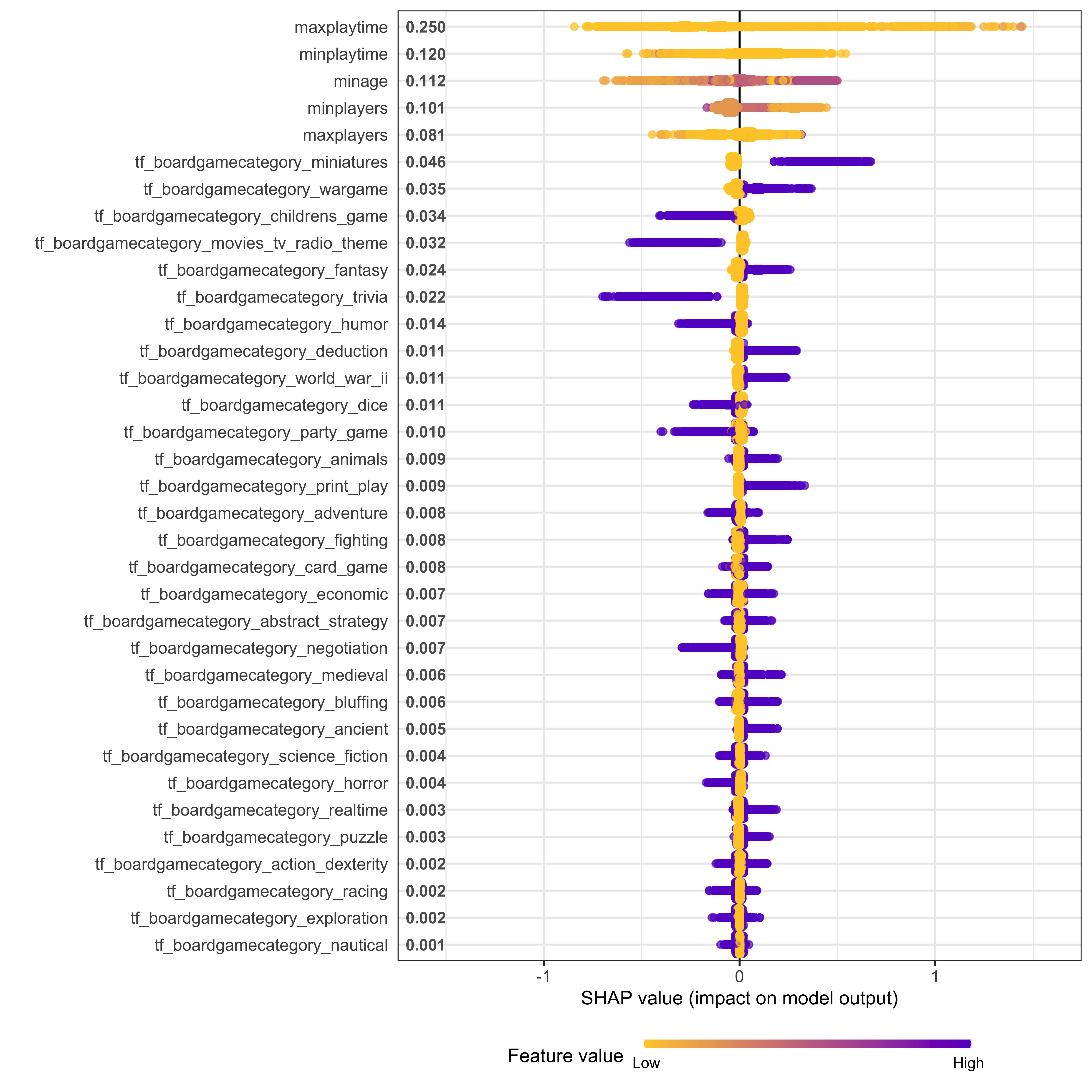
Now we can make visualizations! We can look at an overall summary:

shap.plot.summary(game_shap)

Or create partial dependence plots for specific variables:

shap.plot.dependence(
  game_shap,
  x = "minage",
  color_feature = "minplayers",
  size0 = 1.2,
  smooth = FALSE, add_hist = TRUE
)

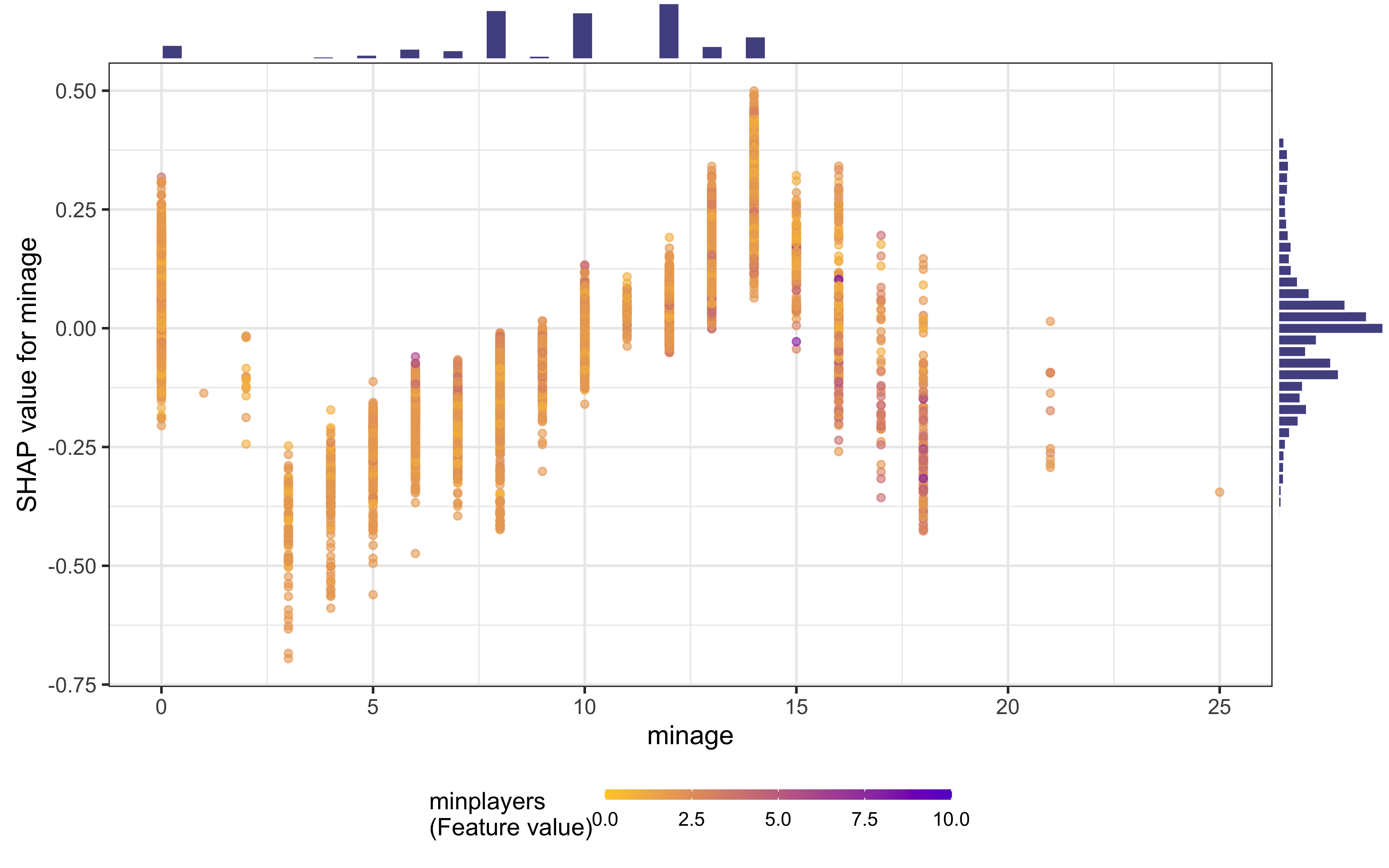
Learning this kind of complex, non-linear behavior is where xgboost models shine.