PCA and UMAP with tidymodels and #TidyTuesday cocktail recipes
By Julia Silge in rstats tidymodels
May 27, 2020
Lately I’ve been publishing
screencasts demonstrating how to use the
tidymodels framework, from first steps in modeling to how to evaluate complex models. Today’s screencast isn’t about predictive modeling, but about unsupervised machine learning using with this week’s
#TidyTuesday dataset on cocktail recipes. 🍸
Here is the code I used in the video, for those who prefer reading instead of or in addition to video.
Explore the data
Our modeling goal is to use unsupervised algorithms for dimensionality reduction with cocktail recipes from this week’s #TidyTuesday dataset. In my earlier blog post this week, I used one of the cocktail datasets included and here let’s use the other one.
boston_cocktails <- readr::read_csv("https://raw.githubusercontent.com/rfordatascience/tidytuesday/master/data/2020/2020-05-26/boston_cocktails.csv")

boston_cocktails %>%
  count(ingredient, sort = TRUE)
## # A tibble: 569 x 2
##    ingredient            n
##    <chr>             <int>
##  1 Gin                 176
##  2 Fresh lemon juice   138
##  3 Simple Syrup        115
##  4 Vodka               114
##  5 Light Rum           113
##  6 Dry Vermouth        107
##  7 Fresh Lime Juice    107
##  8 Triple Sec          107
##  9 Powdered Sugar       90
## 10 Grenadine            85
## # … with 559 more rows
There’s a bit of data cleaning to do to start, both for the ingredient column and the measure column.
cocktails_parsed <- boston_cocktails %>%
  mutate(
    ingredient = str_to_lower(ingredient),
    ingredient = str_replace_all(ingredient, "-", " "),
    ingredient = str_remove(ingredient, " liqueur$"),
    ingredient = str_remove(ingredient, " (if desired)$"),
    ingredient = case_when(
      str_detect(ingredient, "bitters") ~ "bitters",
      str_detect(ingredient, "lemon") ~ "lemon juice",
      str_detect(ingredient, "lime") ~ "lime juice",
      str_detect(ingredient, "grapefruit") ~ "grapefruit juice",
      str_detect(ingredient, "orange") ~ "orange juice",
      TRUE ~ ingredient
    ),
    measure = case_when(
      str_detect(ingredient, "bitters") ~ str_replace(measure, "oz$", "dash"),
      TRUE ~ measure
    ),
    measure = str_replace(measure, " ?1/2", ".5"),
    measure = str_replace(measure, " ?3/4", ".75"),
    measure = str_replace(measure, " ?1/4", ".25"),
    measure_number = parse_number(measure),
    measure_number = if_else(str_detect(measure, "dash$"),
      measure_number / 50,
      measure_number
    )
  ) %>%
  add_count(ingredient) %>%
  filter(n > 15) %>%
  select(-n) %>%
  distinct(row_id, ingredient, .keep_all = TRUE) %>%
  na.omit()

cocktails_parsed
## # A tibble: 2,542 x 7
##    name     category   row_id ingredient_numb… ingredient measure measure_number
##    <chr>    <chr>       <dbl>            <dbl> <chr>      <chr>            <dbl>
##  1 Gauguin  Cocktail …      1                1 light rum  2 oz              2
##  2 Gauguin  Cocktail …      1                3 lemon jui… 1 oz              1
##  3 Gauguin  Cocktail …      1                4 lime juice 1 oz              1
##  4 Fort La… Cocktail …      2                1 light rum  1.5 oz            1.5
##  5 Fort La… Cocktail …      2                2 sweet ver… .5 oz             0.5
##  6 Fort La… Cocktail …      2                3 orange ju… .25 oz            0.25
##  7 Fort La… Cocktail …      2                4 lime juice .25 oz            0.25
##  8 Cuban C… Cocktail …      4                1 lime juice .5 oz             0.5
##  9 Cuban C… Cocktail …      4                2 powdered … .5 oz             0.5
## 10 Cuban C… Cocktail …      4                3 light rum  2 oz              2
## # … with 2,532 more rows
I typically do my data cleaning with data in a tidy format, like boston_cocktails or cocktails_parsed. When it’s time for modeling, we usually need the data in a wider format, so let’s use pivot_wider() to reshape our data.
cocktails_df <- cocktails_parsed %>%
  select(-ingredient_number, -row_id, -measure) %>%
  pivot_wider(names_from = ingredient, values_from = measure_number, values_fill = 0) %>%
  janitor::clean_names() %>%
  na.omit()

cocktails_df
## # A tibble: 937 x 42
##    name  category light_rum lemon_juice lime_juice sweet_vermouth orange_juice
##    <chr> <chr>        <dbl>       <dbl>      <dbl>          <dbl>        <dbl>
##  1 Gaug… Cocktai…      2           1          1               0           0
##  2 Fort… Cocktai…      1.5         0          0.25            0.5         0.25
##  3 Cuba… Cocktai…      2           0          0.5             0           0
##  4 Cool… Cocktai…      0           0          0               0           1
##  5 John… Whiskies      0           1          0               0           0
##  6 Cher… Cocktai…      1.25        0          0               0           0
##  7 Casa… Cocktai…      2           0          1.5             0           0
##  8 Cari… Cocktai…      0.5         0          0               0           0
##  9 Ambe… Cordial…      0           0.25       0               0           0
## 10 The … Whiskies      0           0.5        0               0           0
## # … with 927 more rows, and 35 more variables: powdered_sugar <dbl>,
## #   dark_rum <dbl>, cranberry_juice <dbl>, pineapple_juice <dbl>,
## #   bourbon_whiskey <dbl>, simple_syrup <dbl>, cherry_flavored_brandy <dbl>,
## #   light_cream <dbl>, triple_sec <dbl>, maraschino <dbl>, amaretto <dbl>,
## #   grenadine <dbl>, apple_brandy <dbl>, brandy <dbl>, gin <dbl>,
## #   anisette <dbl>, dry_vermouth <dbl>, apricot_flavored_brandy <dbl>,
## #   bitters <dbl>, straight_rye_whiskey <dbl>, benedictine <dbl>,
## #   egg_white <dbl>, half_and_half <dbl>, vodka <dbl>, grapefruit_juice <dbl>,
## #   blended_scotch_whiskey <dbl>, port <dbl>, white_creme_de_cacao <dbl>,
## #   citrus_flavored_vodka <dbl>, whole_egg <dbl>, egg_yolk <dbl>,
## #   blended_whiskey <dbl>, dubonnet <dbl>, blanco_tequila <dbl>,
## #   old_mr_boston_dry_gin <dbl>
There are lots more great examples of #TidyTuesday EDA out there to explore on Twitter!
Principal component analysis
This dataset is especially delightful because we get to use recipes with recipes. 😍 Let’s load the tidymodels metapackage and implement principal component analysis with a recipe.
library(tidymodels)

pca_rec <- recipe(~., data = cocktails_df) %>%
  update_role(name, category, new_role = "id") %>%
  step_normalize(all_predictors()) %>%
  step_pca(all_predictors())

pca_prep <- prep(pca_rec)

pca_prep
## Data Recipe
##
## Inputs:
##
##       role #variables
##         id          2
##  predictor         40
##
## Training data contained 937 data points and no missing data.
##
## Operations:
##
## Centering and scaling for light_rum, lemon_juice, ... [trained]
## PCA extraction with light_rum, lemon_juice, ... [trained]
Let’s walk through the steps in this recipe.
- First, we must tell the
recipe()what’s going on with our model (notice the formula with no outcome) and what data we are using. - Next, we update the role for cocktail name and category, since these are variables we want to keep around for convenience as identifiers for rows but are not a predictor or outcome.
- We need to center and scale the numeric predictors, because we are about to implement PCA.
- Finally, we use
step_pca()for the actual principal component analysis.
Before using prep() these steps have been defined but not actually run or implemented. The prep() function is where everything gets evaluated.
Once we have that done, we can both explore the results of the PCA. Let’s start with checking out how the PCA turned out. We can tidy() any of our recipe steps, including the PCA step, which is the second step. Then let’s make a visualization to see what the components look like.
tidied_pca <- tidy(pca_prep, 2)

tidied_pca %>%
  filter(component %in% paste0("PC", 1:5)) %>%
  mutate(component = fct_inorder(component)) %>%
  ggplot(aes(value, terms, fill = terms)) +
  geom_col(show.legend = FALSE) +
  facet_wrap(~component, nrow = 1) +
  labs(y = NULL)
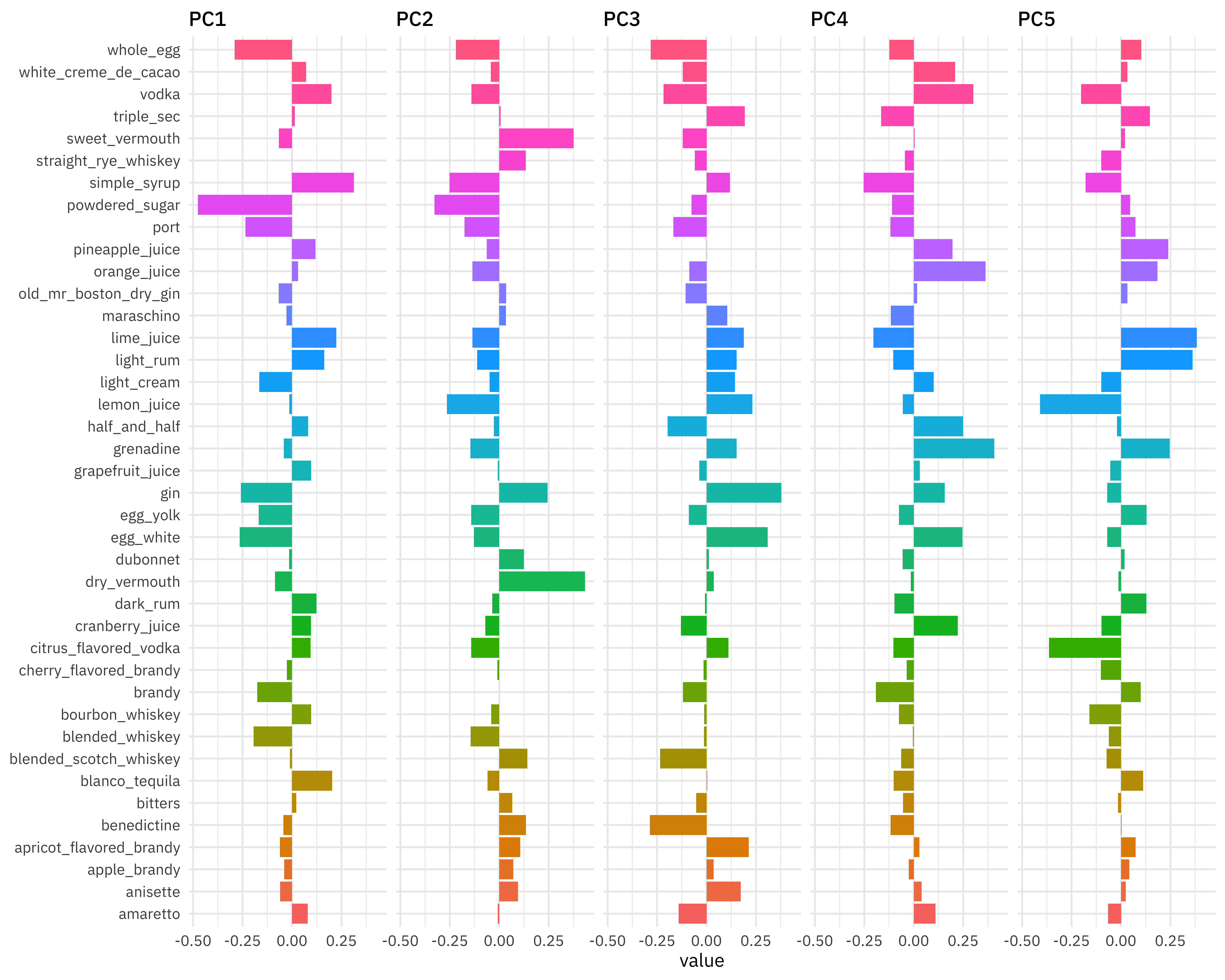
The biggest difference in PC1 is powdered sugar vs. simple syrup; recipes are not likely to have both, which makes sense! Let’s zoom in on the first four components, and understand which cocktail ingredients contribute in the positive and negative directions.
library(tidytext)

tidied_pca %>%
  filter(component %in% paste0("PC", 1:4)) %>%
  group_by(component) %>%
  top_n(8, abs(value)) %>%
  ungroup() %>%
  mutate(terms = reorder_within(terms, abs(value), component)) %>%
  ggplot(aes(abs(value), terms, fill = value > 0)) +
  geom_col() +
  facet_wrap(~component, scales = "free_y") +
  scale_y_reordered() +
  labs(
    x = "Absolute value of contribution",
    y = NULL, fill = "Positive?"
  )
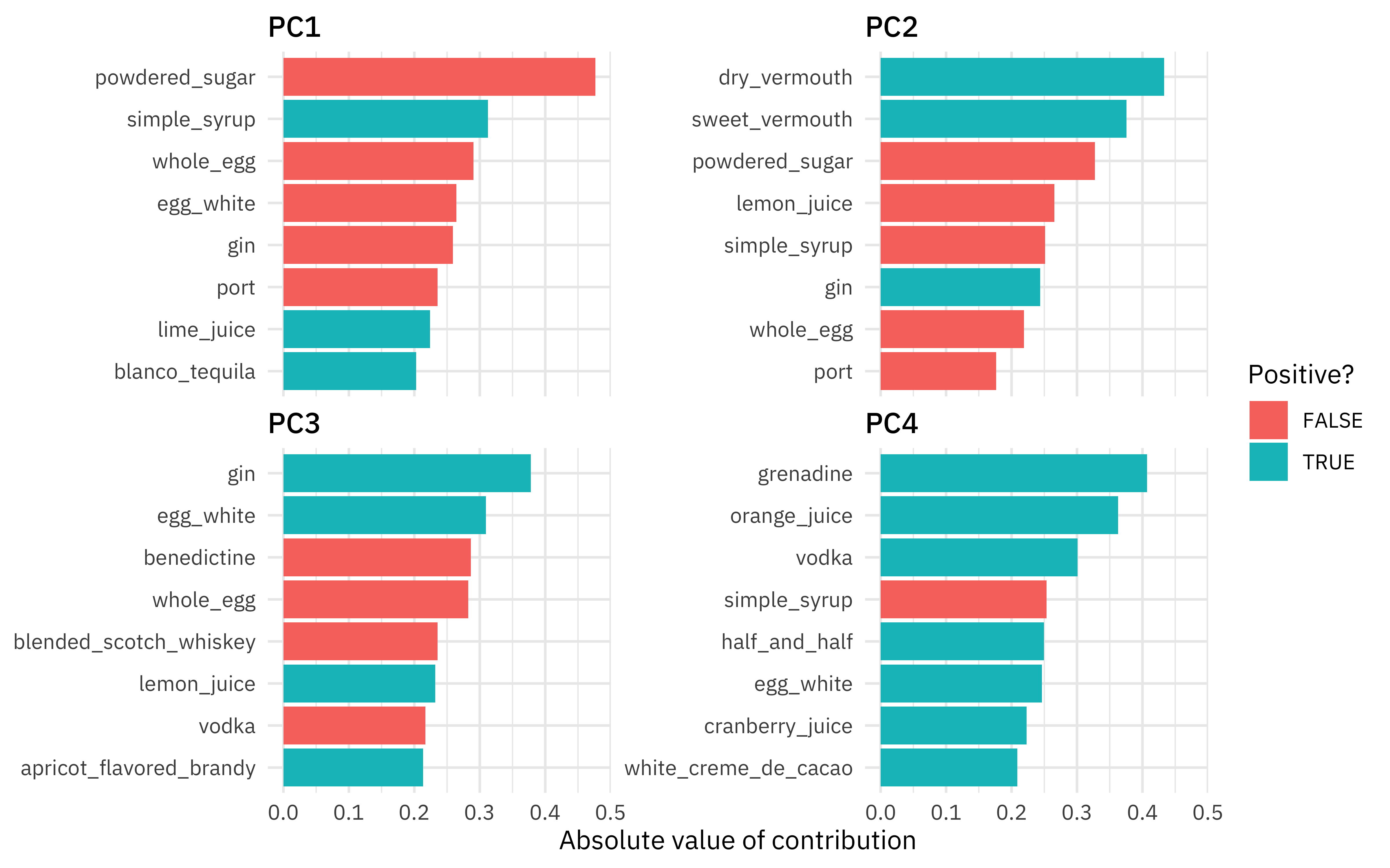
So PC1 is about powdered sugar + egg + gin drinks vs. simple syrup + lime + tequila drinks. This is the component that explains the most variation in drinks. PC2 is mostly about vermouth, both sweet and dry.
How are the cocktails distributed in the plane of the first two components?
juice(pca_prep) %>%
  ggplot(aes(PC1, PC2, label = name)) +
  geom_point(aes(color = category), alpha = 0.7, size = 2) +
  geom_text(check_overlap = TRUE, hjust = "inward", family = "IBMPlexSans") +
  labs(color = NULL)
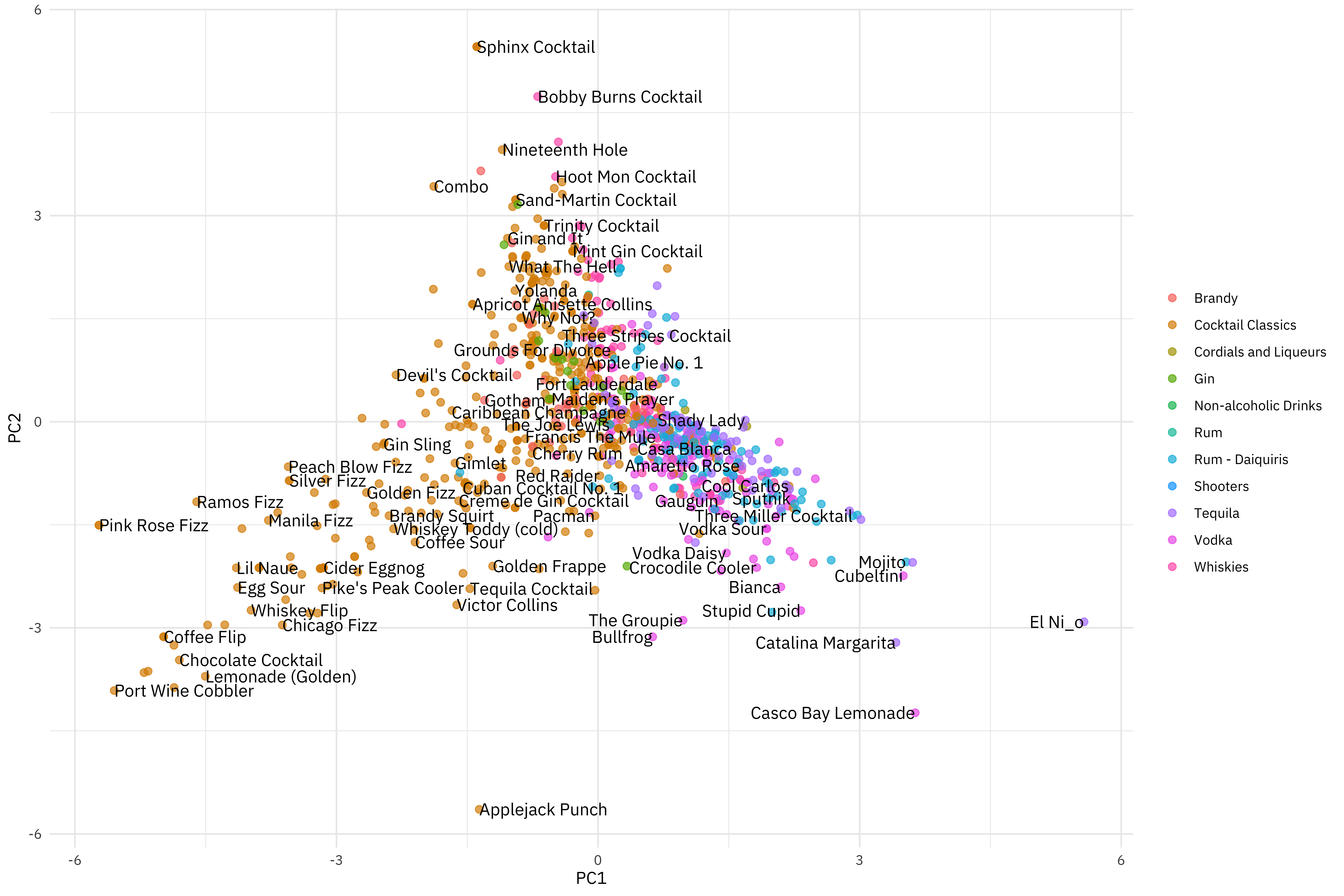
- Fizzy, egg, powdered sugar drinks are to the left.
- Simple syrup, lime, tequila drinks are to the right.
- Vermouth drinks are more to the top.
You can change out PC2 for PC4, for example, to instead see where drinks with more grenadine are.
UMAP
One of the benefits of the tidymodels ecosystem is the flexibility and ease of trying different approaches for the same kind of task. For example, we can switch out PCA for UMAP, an entirely different algorithm for dimensionality reduction based on ideas from topological data analysis. The embed package provides recipe steps for ways to create embeddings including UMAP. Let’s switch out the PCA step for the UMAP step.
library(embed)

umap_rec <- recipe(~., data = cocktails_df) %>%
  update_role(name, category, new_role = "id") %>%
  step_normalize(all_predictors()) %>%
  step_umap(all_predictors())

umap_prep <- prep(umap_rec)

umap_prep
## Data Recipe
##
## Inputs:
##
##       role #variables
##         id          2
##  predictor         40
##
## Training data contained 937 data points and no missing data.
##
## Operations:
##
## Centering and scaling for light_rum, lemon_juice, ... [trained]
## UMAP embedding for light_rum, lemon_juice, ... [trained]
Now we can example how the cocktails are distributed in the plane of the first two UMAP components.
juice(umap_prep) %>%
  ggplot(aes(umap_1, umap_2, label = name)) +
  geom_point(aes(color = category), alpha = 0.7, size = 2) +
  geom_text(check_overlap = TRUE, hjust = "inward", family = "IBMPlexSans") +
  labs(color = NULL)
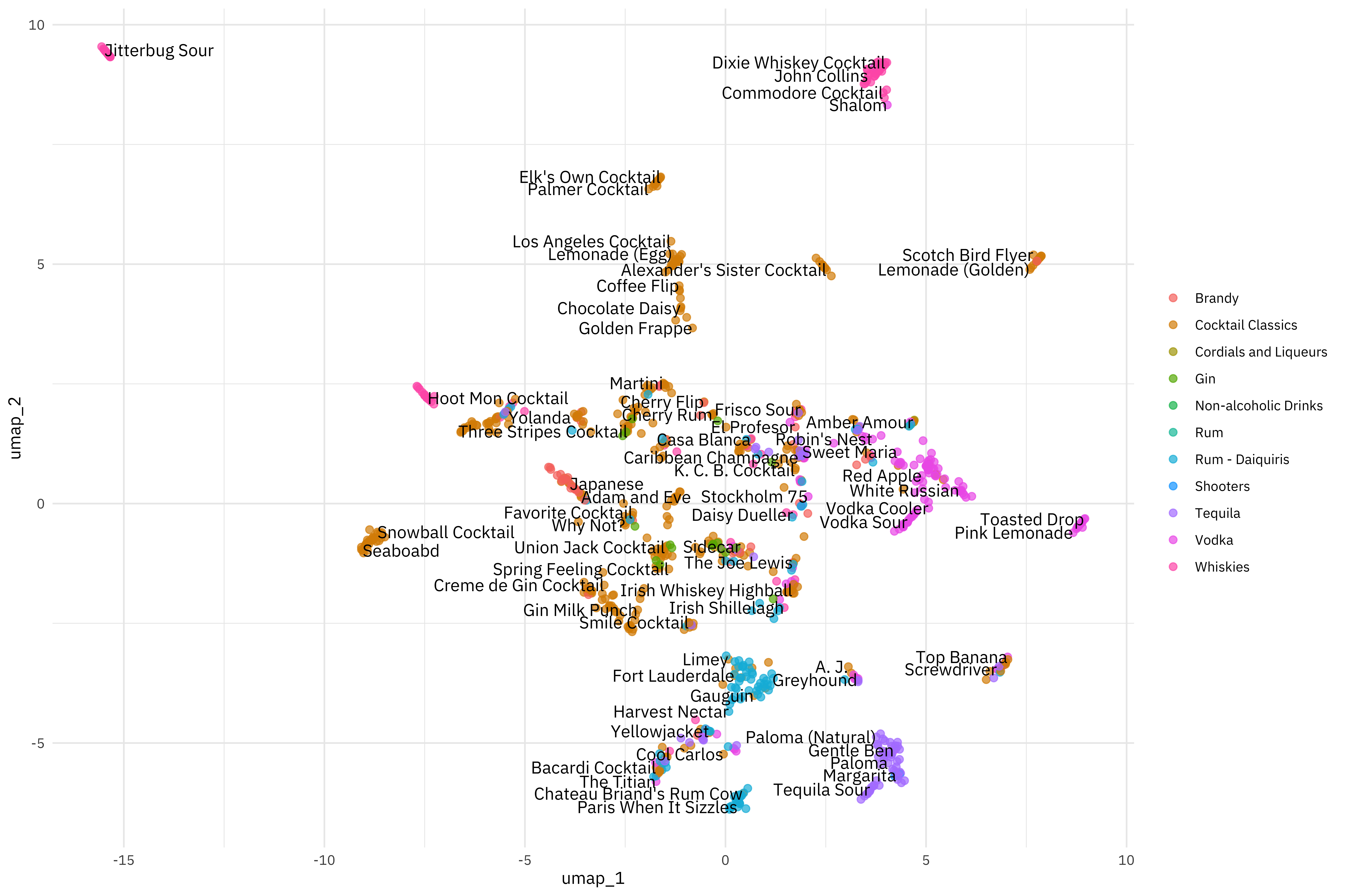
Really interesting, but also different! This is because UMAP is so different from PCA, although they are both approaching this question of how to project a set of features, like ingredients in cocktail recipes, into a smaller space.
- Posted on:
- May 27, 2020
- Length:
- 8 minute read, 1516 words
- Categories:
- rstats tidymodels
- Tags:
- rstats tidymodels