We Are Not Very Evenly Distributed

I saw this tweet making the rounds this past week.

Half of all Americans live in the red counties, half live in the orange counties pic.twitter.com/ptBXNbzSFQ

— Conrad Hackett (@conradhackett) August 8, 2016

Interesting! I saw people using this map to make the argument that the Electoral College was super important, or a terrible idea, or any of a number of other sociopolitical thoughts. This map certainly caught my attention and made me want to know more about this kind of population density distribution.

Census Population Data

I use Census data from the American Community Survey a lot for my work, so let’s get the ACS population estimates for all the counties in the United States. I’m going to use the most recent 5-year estimates, and let’s do some munging so we have FIPS codes for the mapping. (If you haven’t used the acs package before, you will need to get an API key and run api.key.install() one time to install your key on your system.)

library(acs)
library(dplyr)
library(reshape2)
library(stringr)
countygeo <- geo.make(state = "*", county = "*")
popfetch <- acs.fetch(geography = countygeo, 
                      endyear = 2014,
                      span = 5, 
                      table.number = "B01003",
                      col.names = "pretty")
myfips <- geography(popfetch) %>%  
        mutate(fips = str_c(str_pad(state, 2, "left", "0"),
                            str_pad(county, 3, "left", "0"))) %>%
        select(fips)
geography(popfetch)=cbind(myfips, geography(popfetch))
popDF <- melt(estimate(popfetch)) %>%
        mutate(fips = str_sub(str_c("00", Var1), -5),
               pop2014 = value) %>%
        select(fips, pop2014)
head(popDF)

##    fips pop2014
## 1 01001   55136
## 2 01003  191205
## 3 01005   27119
## 4 01007   22653
## 5 01009   57645
## 6 01011   10693

There! Now we have the population in each county.

Making Some Maps

For the mapping, I’m going to use Bob Rudis' albersusa package. It has some really nice map projections for the United States and was great to work with. It turns out that Bob did package up some population numbers with the maps, but we’ll use our ACS data here instead.

library(ggplot2)
library(ggthemes)
library(ggalt)
library(scales)
library(rgeos)
library(maptools)
library(albersusa)
counties <- counties_composite()
counties@data <- left_join(counties@data, popDF, by = "fips")
cmap <- fortify(counties_composite(), region="fips")
ggplot() +
        geom_map(data = cmap, map = cmap,
                    aes(x = long, y = lat, map_id = id),
                    color = "#2b2b2b", size = 0.05, fill = NA) +
        geom_map(data = counties@data, map = cmap,
                 aes(fill = pop2014, map_id = fips),
                 color = NA) +
        theme_map(base_family = "RobotoCondensed-Regular", base_size = 12) +
        theme(plot.title=element_text(family="Roboto-Bold", size = 16, margin=margin(b=10))) +
        theme(plot.subtitle=element_text(size = 14, margin=margin(b=-20))) +
        theme(plot.caption=element_text(size = 9, margin=margin(t=-15))) +
        coord_proj(us_laea_proj) +
        labs(title="Population in U.S. Counties",
             subtitle="Most counties in the United States are sparsely populated",
             caption="ACS Five-Year Estimate 2010-2014") +
        scale_fill_gradient(name = "Population", labels = comma,
                            low = "lavenderblush3", high = "#132B43") +
        theme(legend.position = c(0.8, 0.25))

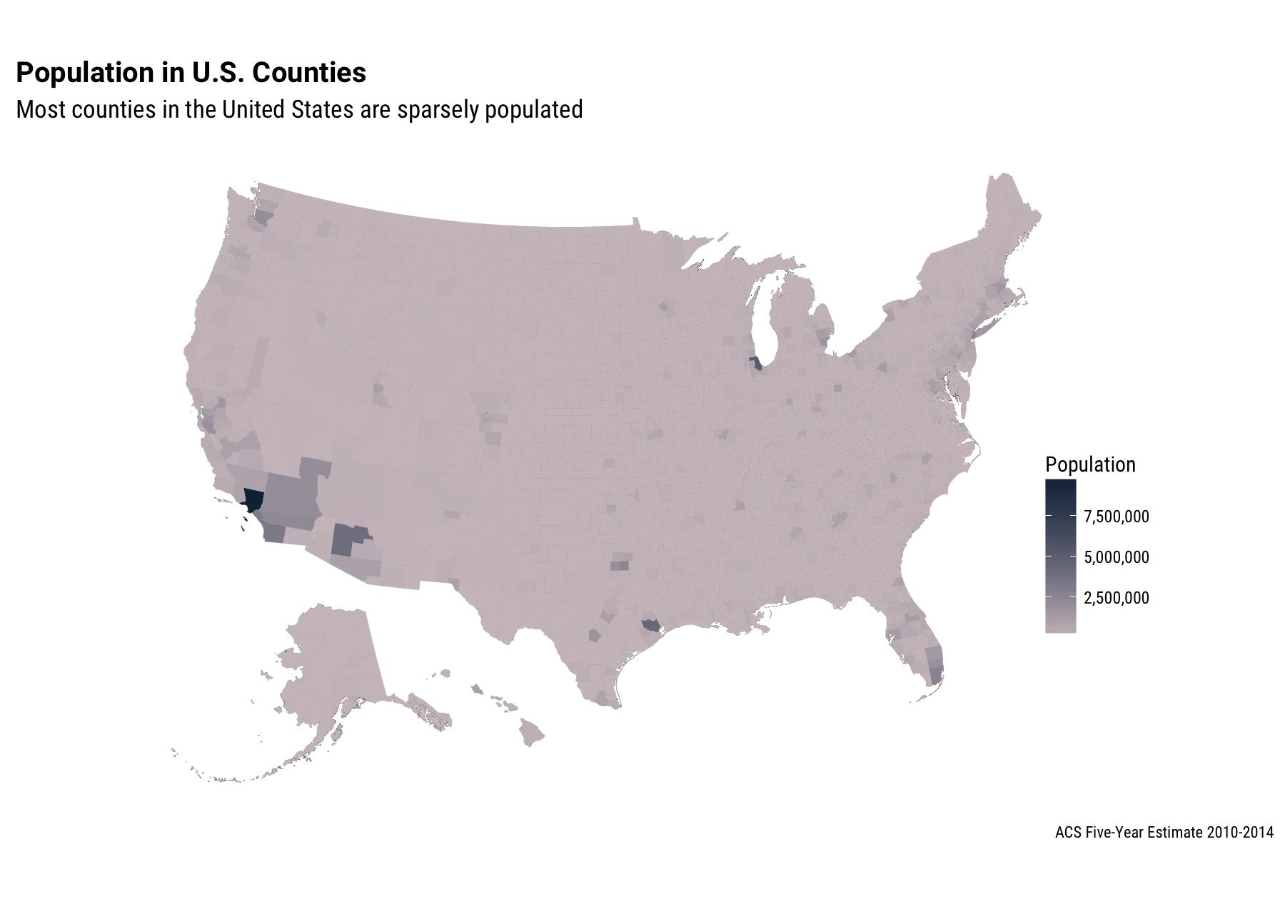
Here we already see how unevenly the U.S. population is distributed. There are almost 10 million people in Los Angeles County, while other large cities like Dallas, Houston, Chicago, and New York are just barely visible with this linear color mapping.

Now we want to find the most populous counties where the top half of the U.S. population lives. Let’s make a copy of the data frame that we’ve used for the mapping, find the total population (and check it, just for sanity’s sake), sort the data frame by population, and then calculate a cumulative sum for the population.

sortingDF <- counties@data %>% select(fips, name, state, pop2014)
totalpop <- sum(sortingDF$pop2014, na.rm = TRUE)
totalpop

## [1] 314107084

sortingDF <- sortingDF %>% arrange(pop2014) %>% 
        mutate(cumsum = cumsum(pop2014))
head(sortingDF, 15)

##     fips      name      state pop2014 cumsum
## 1  15005   Kalawao     Hawaii      73     73
## 2  48301    Loving      Texas      89    162
## 3  48269      King      Texas     290    452
## 4  31117 McPherson   Nebraska     426    878
## 5  31005    Arthur   Nebraska     476   1354
## 6  30069 Petroleum    Montana     489   1843
## 7  48261    Kenedy      Texas     528   2371
## 8  31115      Loup   Nebraska     559   2930
## 9  31009    Blaine   Nebraska     594   3524
## 10 02282   Yakutat     Alaska     635   4159
## 11 48311  McMullen      Texas     646   4805
## 12 31075     Grant   Nebraska     649   5454
## 13 08111  San Juan   Colorado     653   6107
## 14 35021   Harding New Mexico     655   6762
## 15 48033    Borden      Texas     676   7438

Those are some SMALL counties. WOW. Where is the halfway point, i.e., the point where the cumulative sum goes from being less than half of the total population to more than half?

sortingDF <- sortingDF %>% 
        mutate(lowhigh = ifelse(cumsum < totalpop * 0.5, "low", "high")) %>%
        select(fips, lowhigh)
counties@data <- left_join(counties@data, sortingDF, by = "fips")

Now let’s map it.

ggplot() +
        geom_map(data = cmap, map = cmap,
                    aes(x = long, y = lat, map_id = id),
                    color = NA, size = 0.05, fill = NA) +
        geom_map(data = counties@data, map = cmap,
                 aes(fill = lowhigh, map_id = fips),
                 color = NA) +
        theme_map(base_family = "RobotoCondensed-Regular", base_size = 12) +
        theme(plot.title=element_text(family="Roboto-Bold", size = 16, margin=margin(b=10))) +
        theme(plot.subtitle=element_text(size = 14, margin=margin(b=-20))) +
        theme(plot.caption=element_text(size = 9, margin=margin(t=-15))) +
        coord_proj(us_laea_proj) +
        labs(title="Population in U.S. Counties",
             subtitle="Half of the population lives in the dark counties, and half in the light",
             caption="ACS Five-Year Estimate 2010-2014") +
        scale_fill_manual(values = c("#003A54", "#B5DDC9"), name="Population") +
        theme(legend.position=c(0.75, 0.25)) +
        theme(legend.key = element_rect(colour = NA))

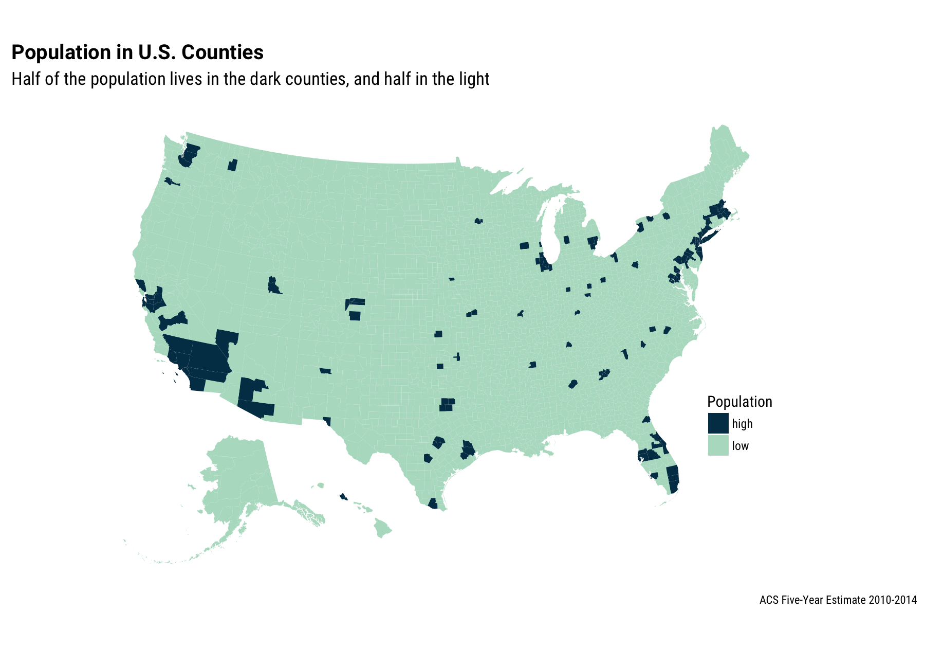
First off, we have exactly reproduced the map in the tweet. This is maybe not entirely surprising because I am pretty sure that the people who made the map in the tweet also used ACS population estimates.

I’ve lived in half a dozen places over the course of my life and I’ve only lived in the darker, high population counties, with the exception of my four years in undergrad that I spent in a pretty small college town. Other than that, I have only lived in the top half of more populous counties. Probably a lot of you have too! That’s what makes them more populous, I suppose.

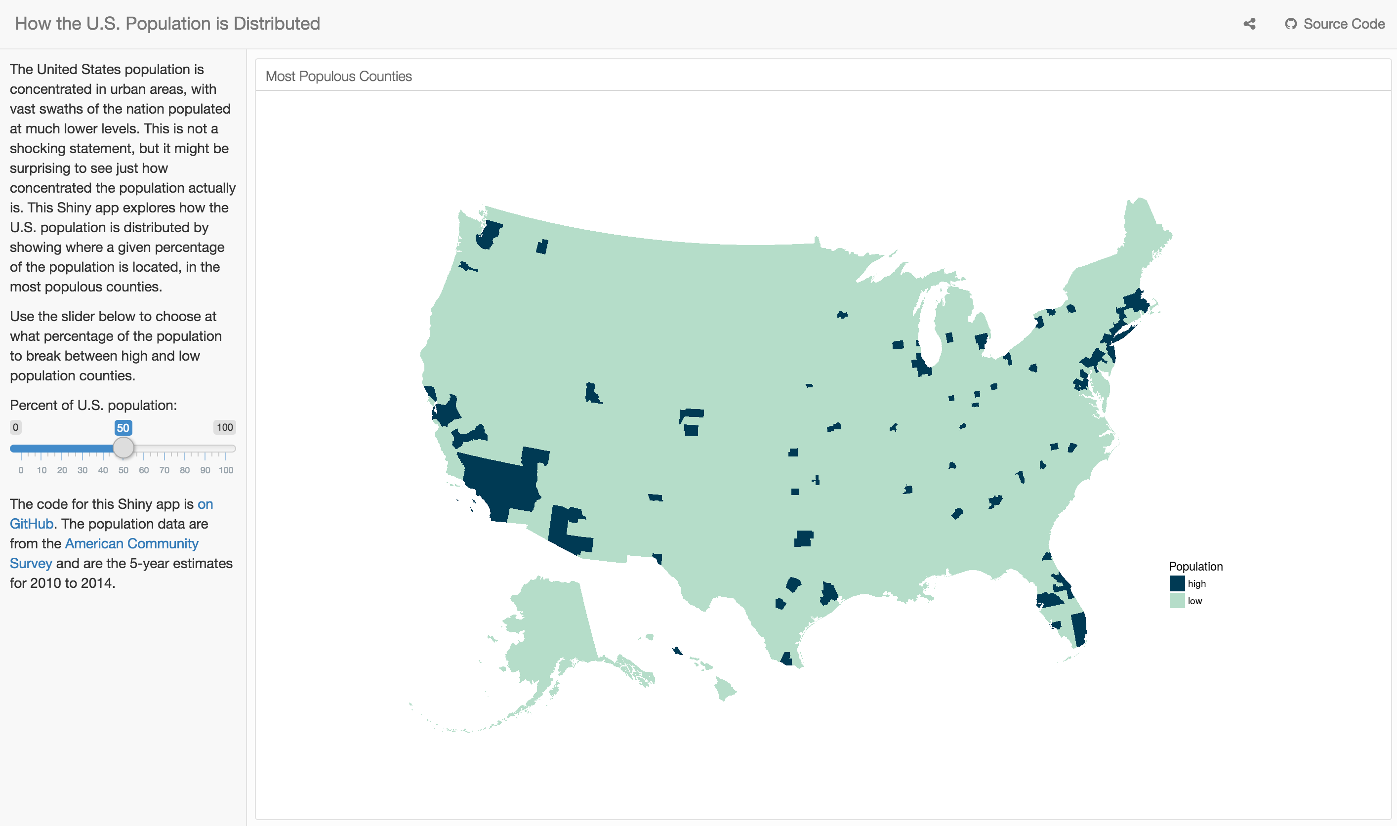
What really motivated me to work on this is that I wanted to be able to learn a bit more about how this population density distribution changes. I made a Shiny app where the user chooses (via a slider) what percentage of the population to use as a break between high and low population counties.

The End

The app is most interesting with the slider between the range of about 30% and 70%, I think; the United States is remarkably urban, at least to me. I would never have argued with someone who told me that the population is concentrated in cities, of course, but the population is more unevenly distributed than I would have predicted. The R Markdown file used to make this blog post is available here. I am very happy to hear feedback or questions!