Modeling #TidyTuesday GDPR violations with tidymodels
By Julia Silge in rstats tidymodels
April 22, 2020
This is an exciting week for us on the tidymodels team; we launched
tidymodels.org, a new central location with resources and documentation for tidymodels packages. There is a TON to explore and learn there! 🚀 You can check out the
official blog post for more details.
Today, I’m publishing here on my blog
another screencast demonstrating how to use tidymodels. This is a good video for folks getting started with tidymodels, using this week’s
#TidyTuesday dataset on GDPR violations. SCARY!!! 😱
Here is the code I used in the video, for those who prefer reading instead of or in addition to video.
Explore the data
Our modeling goal here is to understand what kind of GDPR violations are associated with higher fines in the #TidyTuesday dataset for this week. Before we start, what are the most common GDPR articles actually about? I am not a lawyer, but very roughly:
- Article 5: principles for processing personal data (legitimate purpose, limited)
- Article 6: lawful processing of personal data (i.e. consent, etc)
- Article 13: inform subject when personal data is collected
- Article 15: right of access by data subject
- Article 32: security of processing (i.e. data breaches)
Let’s get started by looking at the data on violations.
library(tidyverse)

gdpr_raw <- readr::read_tsv("https://raw.githubusercontent.com/rfordatascience/tidytuesday/master/data/2020/2020-04-21/gdpr_violations.tsv")

gdpr_raw
## # A tibble: 250 x 11
##       id picture name   price authority date  controller article_violated type
##    <dbl> <chr>   <chr>  <dbl> <chr>     <chr> <chr>      <chr>            <chr>
##  1     1 https:… Pola…   9380 Polish N… 10/1… Polish Ma… Art. 28 GDPR     Non-…
##  2     2 https:… Roma…   2500 Romanian… 10/1… UTTIS IND… Art. 12 GDPR|Ar… Info…
##  3     3 https:… Spain  60000 Spanish … 10/1… Xfera Mov… Art. 5 GDPR|Art… Non-…
##  4     4 https:… Spain   8000 Spanish … 10/1… Iberdrola… Art. 31 GDPR     Fail…
##  5     5 https:… Roma… 150000 Romanian… 10/0… Raiffeise… Art. 32 GDPR     Fail…
##  6     6 https:… Roma…  20000 Romanian… 10/0… Vreau Cre… Art. 32 GDPR|Ar… Fail…
##  7     7 https:… Gree… 200000 Hellenic… 10/0… Telecommu… Art. 5 (1) c) G… Fail…
##  8     8 https:… Gree… 200000 Hellenic… 10/0… Telecommu… Art. 21 (3) GDP… Fail…
##  9     9 https:… Spain  30000 Spanish … 10/0… Vueling A… Art. 5 GDPR|Art… Non-…
## 10    10 https:… Roma…   9000 Romanian… 09/2… Inteligo … Art. 5 (1) a) G… Non-…
## # … with 240 more rows, and 2 more variables: source <chr>, summary <chr>
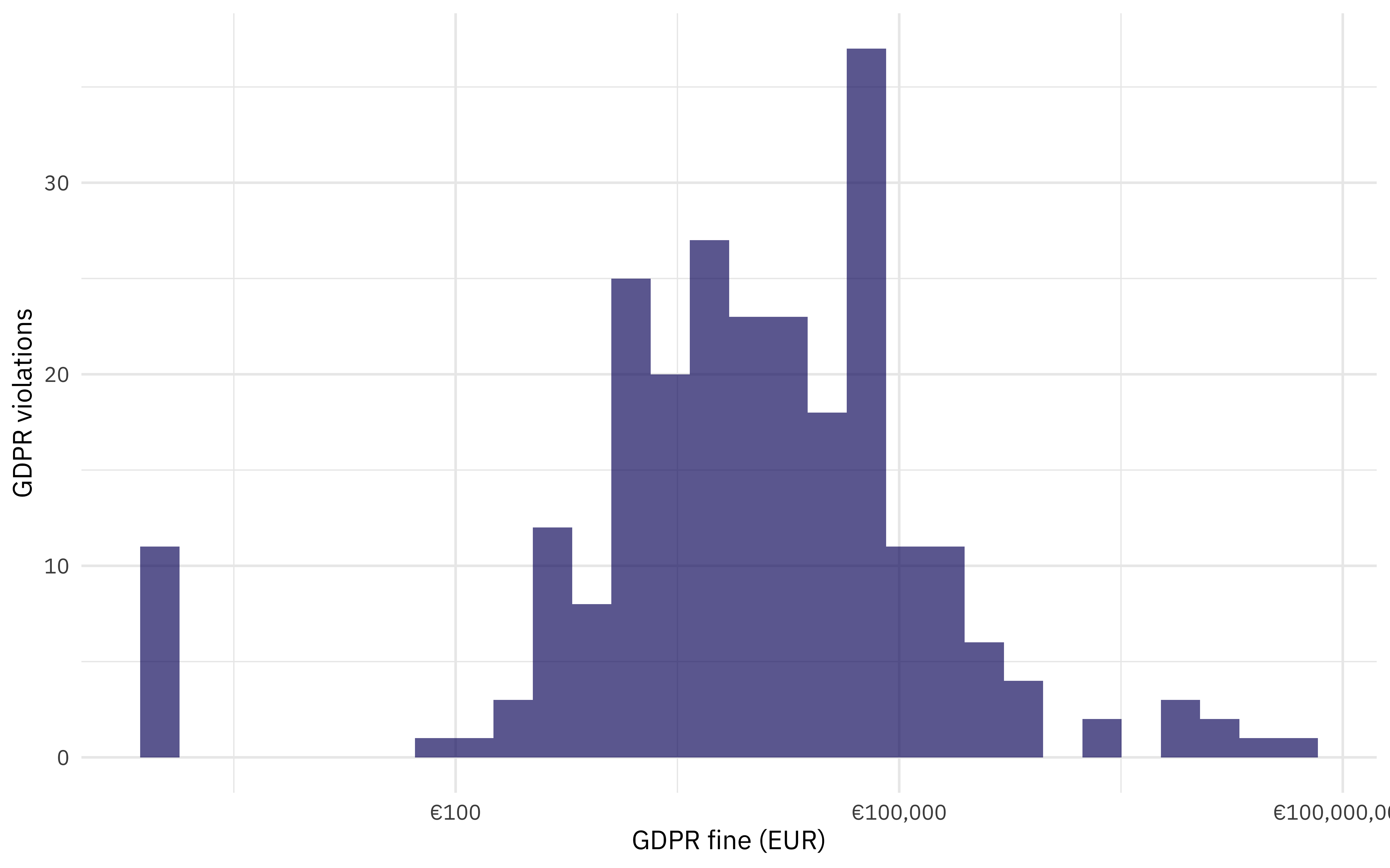
How are the fines distributed?
gdpr_raw %>%
  ggplot(aes(price + 1)) +
  geom_histogram(fill = "midnightblue", alpha = 0.7) +
  scale_x_log10(labels = scales::dollar_format(prefix = "€")) +
  labs(x = "GDPR fine (EUR)", y = "GDPR violations")

Some of the violations were fined zero EUR. Let’s make a one-article-per-row version of this dataset.
gdpr_tidy <- gdpr_raw %>%
  transmute(id,
    price,
    country = name,
    article_violated,
    articles = str_extract_all(article_violated, "Art.[:digit:]+|Art. [:digit:]+")
  ) %>%
  mutate(total_articles = map_int(articles, length)) %>%
  unnest(articles) %>%
  add_count(articles) %>%
  filter(n > 10) %>%
  select(-n)

gdpr_tidy
## # A tibble: 304 x 6
##       id  price country article_violated                 articles total_articles
##    <dbl>  <dbl> <chr>   <chr>                            <chr>             <int>
##  1     2   2500 Romania Art. 12 GDPR|Art. 13 GDPR|Art. … Art. 13               4
##  2     2   2500 Romania Art. 12 GDPR|Art. 13 GDPR|Art. … Art. 5                4
##  3     2   2500 Romania Art. 12 GDPR|Art. 13 GDPR|Art. … Art. 6                4
##  4     3  60000 Spain   Art. 5 GDPR|Art. 6 GDPR          Art. 5                2
##  5     3  60000 Spain   Art. 5 GDPR|Art. 6 GDPR          Art. 6                2
##  6     5 150000 Romania Art. 32 GDPR                     Art. 32               1
##  7     6  20000 Romania Art. 32 GDPR|Art. 33 GDPR        Art. 32               2
##  8     7 200000 Greece  Art. 5 (1) c) GDPR|Art. 25 GDPR  Art. 5                2
##  9     9  30000 Spain   Art. 5 GDPR|Art. 6 GDPR          Art. 5                2
## 10     9  30000 Spain   Art. 5 GDPR|Art. 6 GDPR          Art. 6                2
## # … with 294 more rows
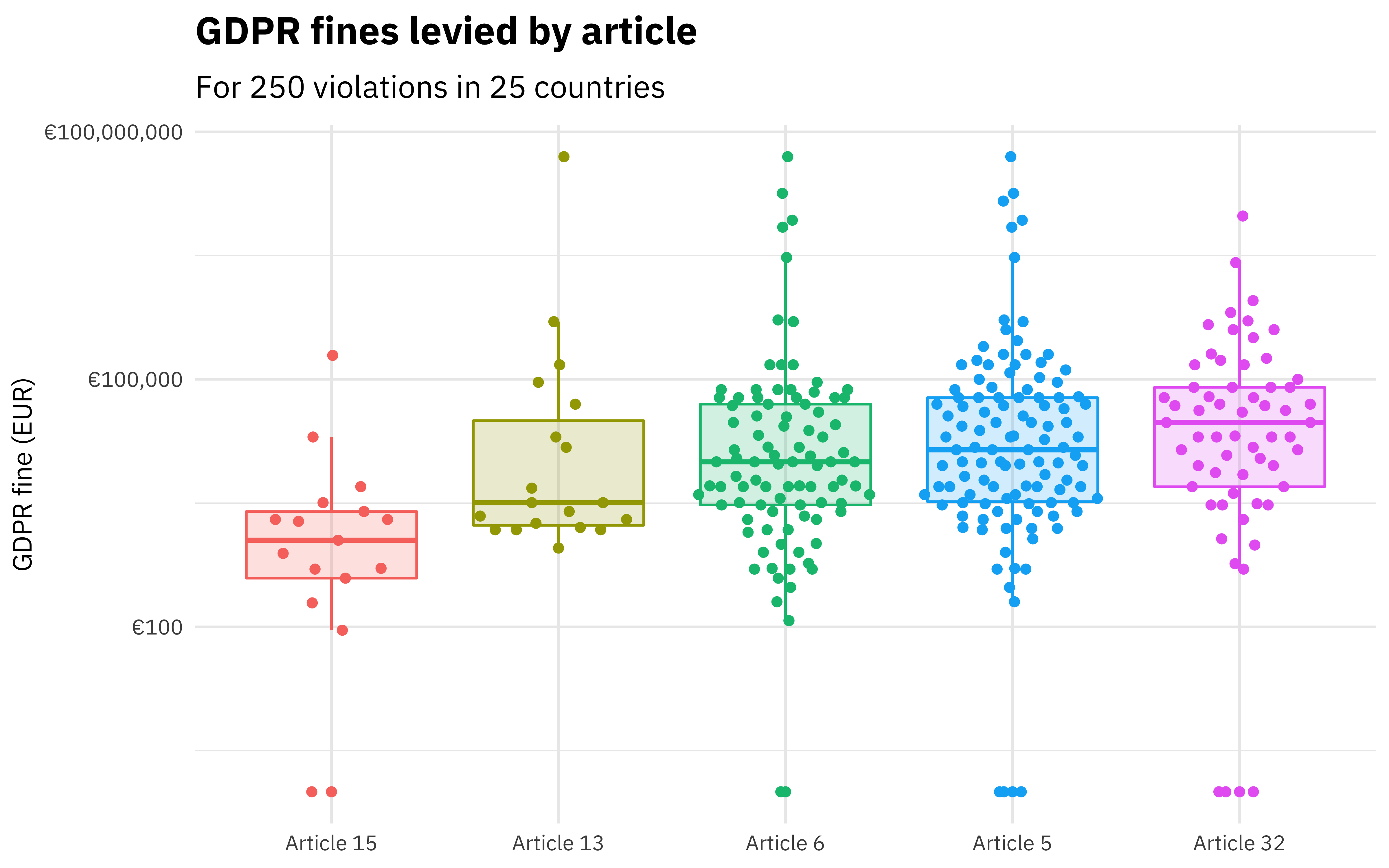
How are the fines distributed by article?
library(ggbeeswarm)

gdpr_tidy %>%
  mutate(
    articles = str_replace_all(articles, "Art. ", "Article "),
    articles = fct_reorder(articles, price)
  ) %>%
  ggplot(aes(articles, price + 1, color = articles, fill = articles)) +
  geom_boxplot(alpha = 0.2, outlier.colour = NA) +
  geom_quasirandom() +
  scale_y_log10(labels = scales::dollar_format(prefix = "€")) +
  labs(
    x = NULL, y = "GDPR fine (EUR)",
    title = "GDPR fines levied by article",
    subtitle = "For 250 violations in 25 countries"
  ) +
  theme(legend.position = "none")

Now let’s create a dataset for modeling.
gdpr_violations <- gdpr_tidy %>%
  mutate(value = 1) %>%
  select(-article_violated) %>%
  pivot_wider(
    names_from = articles, values_from = value,
    values_fn = list(value = max), values_fill = list(value = 0)
  ) %>%
  janitor::clean_names()

gdpr_violations
## # A tibble: 219 x 9
##       id  price country total_articles art_13 art_5 art_6 art_32 art_15
##    <dbl>  <dbl> <chr>            <int>  <dbl> <dbl> <dbl>  <dbl>  <dbl>
##  1     2   2500 Romania              4      1     1     1      0      0
##  2     3  60000 Spain                2      0     1     1      0      0
##  3     5 150000 Romania              1      0     0     0      1      0
##  4     6  20000 Romania              2      0     0     0      1      0
##  5     7 200000 Greece               2      0     1     0      0      0
##  6     9  30000 Spain                2      0     1     1      0      0
##  7    10   9000 Romania              2      0     1     1      0      0
##  8    11 195407 Germany              3      0     0     0      0      1
##  9    12  10000 Belgium              1      0     1     0      0      0
## 10    13 644780 Poland               1      0     0     0      1      0
## # … with 209 more rows
We are ready to go!
Build a model
Let’s preprocess our data to get it ready for modeling.
library(tidymodels)

gdpr_rec <- recipe(price ~ ., data = gdpr_violations) %>%
  update_role(id, new_role = "id") %>%
  step_log(price, base = 10, offset = 1, skip = TRUE) %>%
  step_other(country, other = "Other") %>%
  step_dummy(all_nominal()) %>%
  step_zv(all_predictors())

gdpr_prep <- prep(gdpr_rec)

gdpr_prep
## Data Recipe
##
## Inputs:
##
##       role #variables
##         id          1
##    outcome          1
##  predictor          7
##
## Training data contained 219 data points and no missing data.
##
## Operations:
##
## Log transformation on price [trained]
## Collapsing factor levels for country [trained]
## Dummy variables from country [trained]
## Zero variance filter removed no terms [trained]
Let’s walk through the steps in this recipe.
- First, we must tell the
recipe()what our model is going to be (using a formula here) and what data we are using. - Next, we update the role for
id, since this variable is not a predictor or outcome but I would like to keep it in the data for convenience. - Next, we take the log of the outcome (
price, the amount of the fine). - There are a lot of countries in this dataset, so let’s collapse some of the less frequently occurring countries into another
"Other"category. - Finally, we can create indicator variables and remove varibles with zero variance.
Before using prep() these steps have been defined but not actually run or implemented. The prep() function is where everything gets evaluated.
Now it’s time to specify our model. I am using a
workflow() in this example for convenience; these are objects that can help you manage modeling pipelines more easily, with pieces that fit together like Lego blocks. This workflow() contains both the recipe and the model (a straightforward OLS linear regression).
gdpr_wf <- workflow() %>%
  add_recipe(gdpr_rec) %>%
  add_model(linear_reg() %>%
    set_engine("lm"))

gdpr_wf
## ══ Workflow ═══════════════════════════════════════════════════════════════════════════
## Preprocessor: Recipe
## Model: linear_reg()
##
## ── Preprocessor ───────────────────────────────────────────────────────────────────────
## 4 Recipe Steps
##
## ● step_log()
## ● step_other()
## ● step_dummy()
## ● step_zv()
##
## ── Model ──────────────────────────────────────────────────────────────────────────────
## Linear Regression Model Specification (regression)
##
## Computational engine: lm
You can fit() a workflow, much like you can fit a model, and then you can pull out the fit object and tidy() it!
gdpr_fit <- gdpr_wf %>%
  fit(data = gdpr_violations)

gdpr_fit
## ══ Workflow [trained] ═════════════════════════════════════════════════════════════════
## Preprocessor: Recipe
## Model: linear_reg()
##
## ── Preprocessor ───────────────────────────────────────────────────────────────────────
## 4 Recipe Steps
##
## ● step_log()
## ● step_other()
## ● step_dummy()
## ● step_zv()
##
## ── Model ──────────────────────────────────────────────────────────────────────────────
##
## Call:
## stats::lm(formula = formula, data = data)
##
## Coefficients:
##            (Intercept)          total_articles                  art_13
##                3.76607                 0.47957                -0.76251
##                  art_5                   art_6                  art_32
##               -0.41869                -0.55988                -0.15317
##                 art_15  country_Czech.Republic         country_Germany
##               -1.56765                -0.64953                 0.05974
##        country_Hungary         country_Romania           country_Spain
##               -0.15532                -0.34580                 0.42968
##          country_Other
##                0.23438
gdpr_fit %>%
  pull_workflow_fit() %>%
  tidy() %>%
  arrange(estimate) %>%
  kable()
| term | estimate | std.error | statistic | p.value |
|---|---|---|---|---|
| art_15 | -1.5676538 | 0.4651576 | -3.3701564 | 0.0008969 |
| art_13 | -0.7625069 | 0.4074302 | -1.8715031 | 0.0626929 |
| country_Czech.Republic | -0.6495339 | 0.4667470 | -1.3916188 | 0.1655387 |
| art_6 | -0.5598765 | 0.2950382 | -1.8976404 | 0.0591419 |
| art_5 | -0.4186949 | 0.2828869 | -1.4800789 | 0.1403799 |
| country_Romania | -0.3457980 | 0.4325560 | -0.7994295 | 0.4249622 |
| country_Hungary | -0.1553232 | 0.4790037 | -0.3242631 | 0.7460679 |
| art_32 | -0.1531725 | 0.3146769 | -0.4867613 | 0.6269450 |
| country_Germany | 0.0597408 | 0.4189434 | 0.1425986 | 0.8867465 |
| country_Other | 0.2343787 | 0.3551225 | 0.6599939 | 0.5099950 |
| country_Spain | 0.4296805 | 0.3643060 | 1.1794494 | 0.2395796 |
| total_articles | 0.4795667 | 0.1656494 | 2.8950705 | 0.0041993 |
| (Intercept) | 3.7660677 | 0.4089156 | 9.2098904 | 0.0000000 |
GDPR violations of more than one article have higher fines.
Explore results
Lots of those coefficients have big p-values (for example, all the countries) but I think the best way to understand these results will be to visualize some predictions. You can predict on new data in tidymodels with either a model or a workflow().
Let’s create some example new data that we are interested in.
new_gdpr <- crossing(
  country = "Other",
  art_5 = 0:1,
  art_6 = 0:1,
  art_13 = 0:1,
  art_15 = 0:1,
  art_32 = 0:1
) %>%
  mutate(
    id = row_number(),
    total_articles = art_5 + art_6 + art_13 + art_15 + art_32
  )

new_gdpr
## # A tibble: 32 x 8
##    country art_5 art_6 art_13 art_15 art_32    id total_articles
##    <chr>   <int> <int>  <int>  <int>  <int> <int>          <int>
##  1 Other       0     0      0      0      0     1              0
##  2 Other       0     0      0      0      1     2              1
##  3 Other       0     0      0      1      0     3              1
##  4 Other       0     0      0      1      1     4              2
##  5 Other       0     0      1      0      0     5              1
##  6 Other       0     0      1      0      1     6              2
##  7 Other       0     0      1      1      0     7              2
##  8 Other       0     0      1      1      1     8              3
##  9 Other       0     1      0      0      0     9              1
## 10 Other       0     1      0      0      1    10              2
## # … with 22 more rows
Let’s find both the mean predictions and the confidence intervals.
mean_pred <- predict(gdpr_fit,
  new_data = new_gdpr
)

conf_int_pred <- predict(gdpr_fit,
  new_data = new_gdpr,
  type = "conf_int"
)

gdpr_res <- new_gdpr %>%
  bind_cols(mean_pred) %>%
  bind_cols(conf_int_pred)

gdpr_res
## # A tibble: 32 x 11
##    country art_5 art_6 art_13 art_15 art_32    id total_articles .pred
##    <chr>   <int> <int>  <int>  <int>  <int> <int>          <int> <dbl>
##  1 Other       0     0      0      0      0     1              0  4.00
##  2 Other       0     0      0      0      1     2              1  4.33
##  3 Other       0     0      0      1      0     3              1  2.91
##  4 Other       0     0      0      1      1     4              2  3.24
##  5 Other       0     0      1      0      0     5              1  3.72
##  6 Other       0     0      1      0      1     6              2  4.04
##  7 Other       0     0      1      1      0     7              2  2.63
##  8 Other       0     0      1      1      1     8              3  2.96
##  9 Other       0     1      0      0      0     9              1  3.92
## 10 Other       0     1      0      0      1    10              2  4.25
## # … with 22 more rows, and 2 more variables: .pred_lower <dbl>,
## #   .pred_upper <dbl>
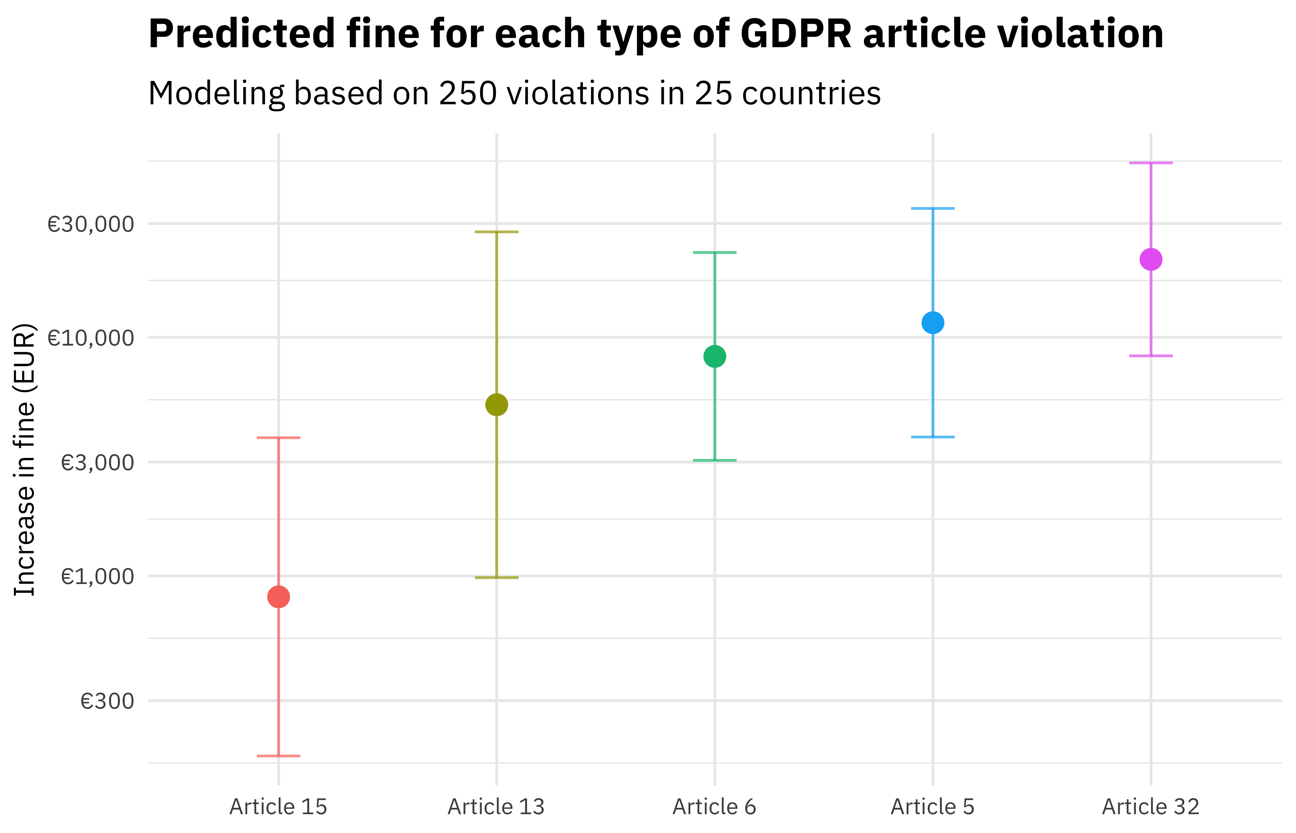
There are lots of things we can do wtih these results! For example, what are the predicted GDPR fines for violations of each article type (violating only one article)?
gdpr_res %>%
  filter(total_articles == 1) %>%
  pivot_longer(art_5:art_32) %>%
  filter(value > 0) %>%
  mutate(
    name = str_replace_all(name, "art_", "Article "),
    name = fct_reorder(name, .pred)
  ) %>%
  ggplot(aes(name, 10^.pred, color = name)) +
  geom_point(size = 3.5) +
  geom_errorbar(aes(
    ymin = 10^.pred_lower,
    ymax = 10^.pred_upper
  ),
  width = 0.2, alpha = 0.7
  ) +
  labs(
    x = NULL, y = "Increase in fine (EUR)",
    title = "Predicted fine for each type of GDPR article violation",
    subtitle = "Modeling based on 250 violations in 25 countries"
  ) +
  scale_y_log10(labels = scales::dollar_format(prefix = "€", accuracy = 1)) +
  theme(legend.position = "none")

We can see here that violations such as data breaches have higher fines on average than violations about rights of access.
- Posted on:
- April 22, 2020
- Length:
- 10 minute read, 2027 words
- Categories:
- rstats tidymodels
- Tags:
- rstats tidymodels