PCA and the #TidyTuesday best hip hop songs ever
By Julia Silge in rstats tidymodels
April 14, 2020
Lately I’ve been publishing
screencasts demonstrating how to use the tidymodels framework, from first steps in modeling to how to tune more complex models. Today, I’m exploring a different part of the tidymodels framework; I’m showing how to implement principal component analysis via recipes with this week’s
#TidyTuesday dataset on the best hip hop songs of all time as determinded by a BBC poll of music critics.
Here is the code I used in the video, for those who prefer reading instead of or in addition to video.
Explore the data
Our modeling goal here is to understand what kind of songs are more highly rated by music critics in the #TidyTuesday dataset on hip hop songs. We’ll use principal component analysis and audio features available in the Spotify API to do this! 🎵
First, let’s look at the data on the rankings.
library(tidyverse)

rankings <- read_csv("https://raw.githubusercontent.com/rfordatascience/tidytuesday/master/data/2020/2020-04-14/rankings.csv")

rankings
## # A tibble: 311 x 12
##       ID title   artist   year gender points     n    n1    n2    n3    n4    n5
##    <dbl> <chr>   <chr>   <dbl> <chr>   <dbl> <dbl> <dbl> <dbl> <dbl> <dbl> <dbl>
##  1     1 Juicy   The No…  1994 male      140    18     9     3     3     1     2
##  2     2 Fight … Public…  1989 male      100    11     7     3     1     0     0
##  3     3 Shook … Mobb D…  1995 male       94    13     4     5     1     1     2
##  4     4 The Me… Grandm…  1982 male       90    14     5     3     1     0     5
##  5     5 Nuthin… Dr Dre…  1992 male       84    14     2     4     2     4     2
##  6     6 C.R.E.… Wu-Tan…  1993 male       62    10     3     1     1     4     1
##  7     7 93 ’Ti… Souls …  1993 male       50     7     2     2     2     0     1
##  8     8 Passin… The Ph…  1992 male       48     6     3     2     0     0     1
##  9     9 N.Y. S… Nas      1994 male       46     7     1     3     1     1     1
## 10    10 Dear M… 2Pac     1995 male       42     6     2     1     1     2     0
## # … with 301 more rows
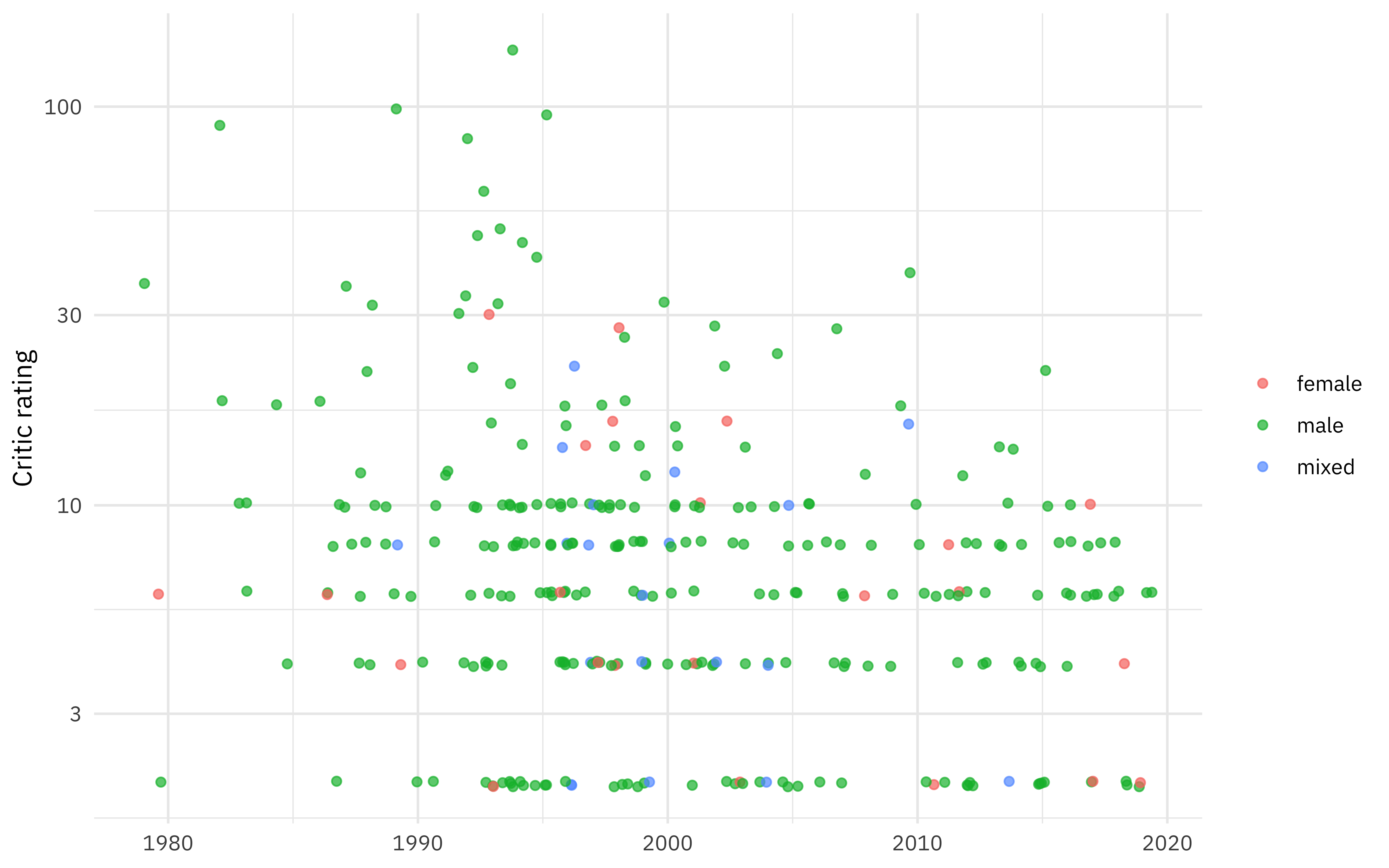
As a first step, let’s recreate the plot from the source material, but adjusted a bit.
rankings %>%
  ggplot(aes(year, points, color = gender)) +
  geom_jitter(alpha = 0.7) +
  scale_y_log10() +
  labs(
    y = "Critic rating",
    x = NULL,
    color = NULL
  )
To see more examples of EDA for this dataset, you can see the great work that folks share on Twitter! ✨ Next, let’s get audio features from the Spotify API.
Get audio features
Spotify makes a set of “audio features” available in its API. This includes features like whether the song is in a major or minor key, the liveness, the instrumentalness, the danceability, and many others. One option to work with these songs would be to get them all at once via a playlist that Tom Mock made.
library(spotifyr)
access_token <- get_spotify_access_token()

playlist_features <- get_playlist_audio_features("tmock1923", "7esD007S7kzeSwVtcH9GFe")

playlist_features
## # A tibble: 250 x 61
##    playlist_id playlist_name playlist_img playlist_owner_… playlist_owner_…
##    <chr>       <chr>         <chr>        <chr>            <chr>
##  1 7esD007S7k… Top 250 Hiph… https://mos… tmock1923        tmock1923
##  2 7esD007S7k… Top 250 Hiph… https://mos… tmock1923        tmock1923
##  3 7esD007S7k… Top 250 Hiph… https://mos… tmock1923        tmock1923
##  4 7esD007S7k… Top 250 Hiph… https://mos… tmock1923        tmock1923
##  5 7esD007S7k… Top 250 Hiph… https://mos… tmock1923        tmock1923
##  6 7esD007S7k… Top 250 Hiph… https://mos… tmock1923        tmock1923
##  7 7esD007S7k… Top 250 Hiph… https://mos… tmock1923        tmock1923
##  8 7esD007S7k… Top 250 Hiph… https://mos… tmock1923        tmock1923
##  9 7esD007S7k… Top 250 Hiph… https://mos… tmock1923        tmock1923
## 10 7esD007S7k… Top 250 Hiph… https://mos… tmock1923        tmock1923
## # … with 240 more rows, and 56 more variables: danceability <dbl>,
## #   energy <dbl>, key <int>, loudness <dbl>, mode <int>, speechiness <dbl>,
## #   acousticness <dbl>, instrumentalness <dbl>, liveness <dbl>, valence <dbl>,
## #   tempo <dbl>, track.id <chr>, analysis_url <chr>, time_signature <int>,
## #   added_at <chr>, is_local <lgl>, primary_color <lgl>, added_by.href <chr>,
## #   added_by.id <chr>, added_by.type <chr>, added_by.uri <chr>,
## #   added_by.external_urls.spotify <chr>, track.artists <list>,
## #   track.available_markets <list>, track.disc_number <int>,
## #   track.duration_ms <int>, track.episode <lgl>, track.explicit <lgl>,
## #   track.href <chr>, track.is_local <lgl>, track.name <chr>,
## #   track.popularity <int>, track.preview_url <chr>, track.track <lgl>,
## #   track.track_number <int>, track.type <chr>, track.uri <chr>,
## #   track.album.album_type <chr>, track.album.artists <list>,
## #   track.album.available_markets <list>, track.album.href <chr>,
## #   track.album.id <chr>, track.album.images <list>, track.album.name <chr>,
## #   track.album.release_date <chr>, track.album.release_date_precision <chr>,
## #   track.album.total_tracks <int>, track.album.type <chr>,
## #   track.album.uri <chr>, track.album.external_urls.spotify <chr>,
## #   track.external_ids.isrc <chr>, track.external_urls.spotify <chr>,
## #   video_thumbnail.url <lgl>, key_name <chr>, mode_name <chr>, key_mode <chr>
This would be perfect for exploring the audio features on their own. On the other hand, this is going to be pretty difficult to match up to the songs in the rankings dataset because both the titles and artists are significantly different, so let’s take a different approach. Let’s create a little function to find the Spotify track identifier via search_spotify() (Spotify has already handled search pretty well) and use purrr::map() to apply it to all the songs we have in our dataset.
pull_id <- function(query) {
  search_spotify(query, "track") %>%
    arrange(-popularity) %>%
    filter(row_number() == 1) %>%
    pull(id)
}

ranking_ids <- rankings %>%
  mutate(
    search_query = paste(title, artist),
    search_query = str_to_lower(search_query),
    search_query = str_remove(search_query, "ft.*$")
  ) %>%
  mutate(id = map_chr(search_query, possibly(pull_id, NA_character_)))

ranking_ids %>%
  select(title, artist, id)
## # A tibble: 311 x 3
##    title                  artist                            id
##    <chr>                  <chr>                             <chr>
##  1 Juicy                  The Notorious B.I.G.              5ByAIlEEnxYdvpnezg7…
##  2 Fight The Power        Public Enemy                      1yo16b3u0lptm6Cs7lx…
##  3 Shook Ones (Part II)   Mobb Deep                         4nASzyRbzL5qZQuOPjQ…
##  4 The Message            Grandmaster Flash & The Furious … 5DuTNKFEjJIySAyJH1y…
##  5 Nuthin’ But A ‘G’ Tha… Dr Dre ft. Snoop Doggy Dogg       4YtoipFgf4k0AfD17Zf…
##  6 C.R.E.A.M.             Wu-Tang Clan                      119c93MHjrDLJTApCVG…
##  7 93 ’Til Infinity       Souls of Mischief                 0PV1TFUMTBrDETzW6KQ…
##  8 Passin’ Me By          The Pharcyde                      4G3dZN9o3o2X4VKwt4C…
##  9 N.Y. State Of Mind     Nas                               5zwz05jkQVT68CjUpPw…
## 10 Dear Mama              2Pac                              6tDxrq4FxEL2q15y37t…
## # … with 301 more rows
At the end of that, there are 6% of songs that I failed to find a Spotify track identifier for. Not too bad!
Now that we have the track identifiers, we can get the audio features. The function get_track_audio_features() can only take 100 tracks at most at once, so let’s divide up our tracks into smaller chunks and then map() through them.
ranking_features <- ranking_ids %>%
  mutate(id_group = row_number() %/% 80) %>%
  select(id_group, id) %>%
  nest(data = c(id)) %>%
  mutate(audio_features = map(data, ~ get_track_audio_features(.$id)))

ranking_features
## # A tibble: 4 x 3
##   id_group data              audio_features
##      <dbl> <list>            <list>
## 1        0 <tibble [79 × 1]> <tibble [79 × 18]>
## 2        1 <tibble [80 × 1]> <tibble [80 × 18]>
## 3        2 <tibble [80 × 1]> <tibble [80 × 18]>
## 4        3 <tibble [72 × 1]> <tibble [72 × 18]>
We have audio features! 🎉 Now let’s put that together with the rankings and create a dataframe for modeling.
ranking_df <- ranking_ids %>%
  bind_cols(ranking_features %>%
    select(audio_features) %>%
    unnest(audio_features)) %>%
  select(title, artist, points, year, danceability:tempo) %>%
  na.omit()

ranking_df
## # A tibble: 293 x 15
##    title artist points  year danceability energy   key loudness  mode
##    <chr> <chr>   <dbl> <dbl>        <dbl>  <dbl> <int>    <dbl> <int>
##  1 Juicy The N…    140  1994        0.889  0.816     9    -4.67     1
##  2 Figh… Publi…    100  1989        0.797  0.582     2   -13.0      1
##  3 Shoo… Mobb …     94  1995        0.637  0.878     6    -5.51     1
##  4 The … Grand…     90  1982        0.947  0.607    10   -10.6      0
##  5 Nuth… Dr Dr…     84  1992        0.801  0.699    11    -8.18     0
##  6 C.R.… Wu-Ta…     62  1993        0.479  0.549    11   -10.6      0
##  7 93 ’… Souls…     50  1993        0.59   0.672     1   -11.8      1
##  8 Pass… The P…     48  1992        0.759  0.756     4    -8.14     0
##  9 N.Y.… Nas        46  1994        0.665  0.91      6    -4.68     0
## 10 Dear… 2Pac       42  1995        0.773  0.54      6    -7.12     1
## # … with 283 more rows, and 6 more variables: speechiness <dbl>,
## #   acousticness <dbl>, instrumentalness <dbl>, liveness <dbl>, valence <dbl>,
## #   tempo <dbl>
How are these quantities correlated with each other?
library(corrr)

ranking_df %>%
  select(year:tempo) %>%
  correlate() %>%
  rearrange() %>%
  shave() %>%
  rplot(shape = 15, colours = c("darkorange", "white", "darkcyan")) +
  theme_plex()
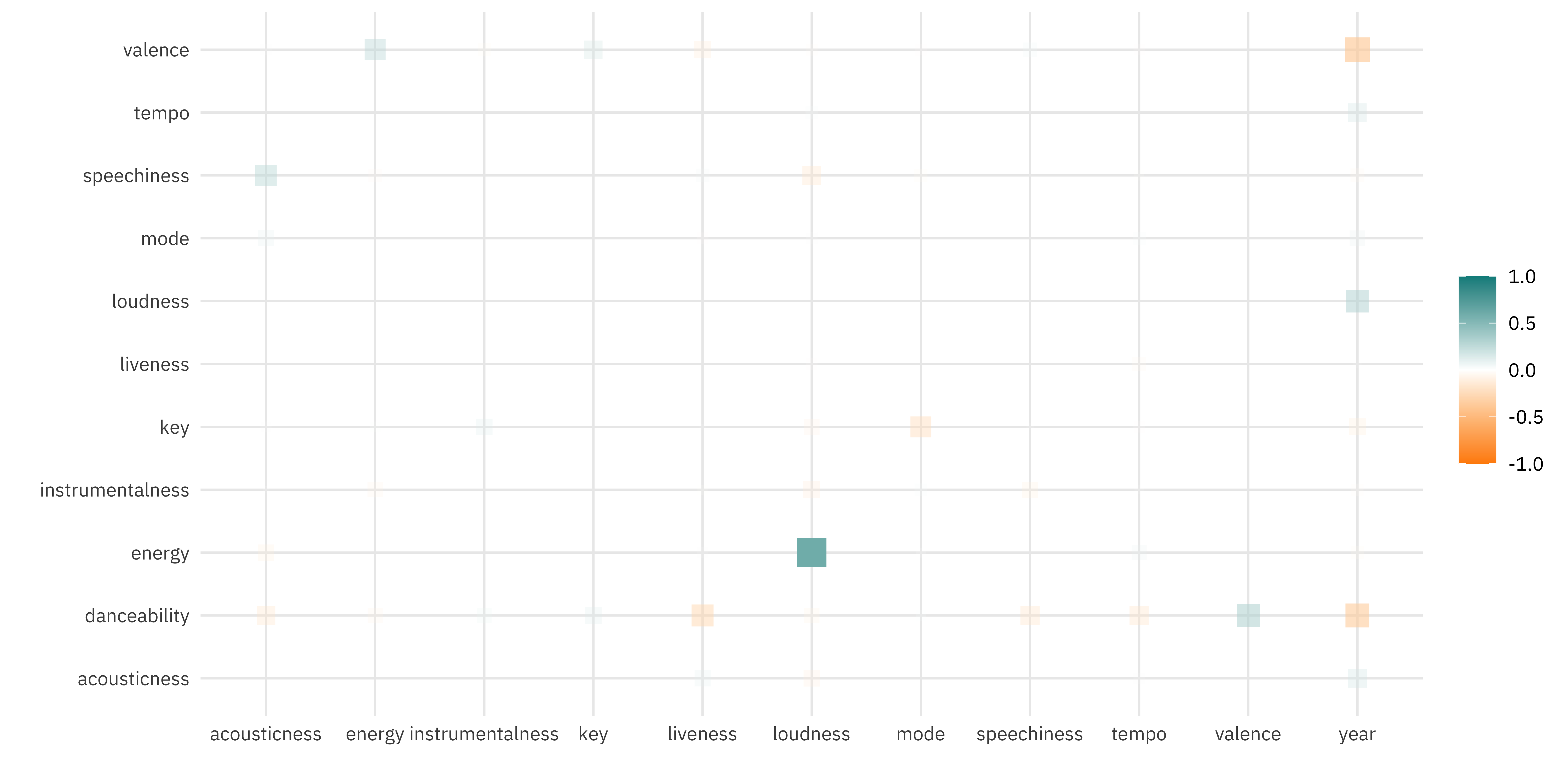
Louder songs have higher energy, and older songs tend to be more danceable and have higher valence (i.e. be more “happy”).
Let’s train a linear model on these audio features.
ranking_lm <- ranking_df %>%
  select(-title, -artist) %>%
  lm(log(points) ~ ., data = .)

summary(ranking_lm)
##
## Call:
## lm(formula = log(points) ~ ., data = .)
##
## Residuals:
##      Min       1Q   Median       3Q      Max
## -1.68521 -0.58721  0.05728  0.44134  2.63178
##
## Coefficients:
##                    Estimate Std. Error t value Pr(>|t|)
## (Intercept)      68.2251604 13.9295818   4.898 1.64e-06 ***
## year             -0.0329381  0.0068396  -4.816 2.40e-06 ***
## danceability      0.0068425  0.4409221   0.016    0.988
## energy           -0.0487288  0.4372164  -0.111    0.911
## key               0.0091604  0.0137126   0.668    0.505
## loudness          0.0360689  0.0226039   1.596    0.112
## mode             -0.0690822  0.1041311  -0.663    0.508
## speechiness      -0.2697032  0.4118937  -0.655    0.513
## acousticness      0.4754636  0.3003998   1.583    0.115
## instrumentalness -0.6862222  0.8101330  -0.847    0.398
## liveness          0.0811289  0.2604150   0.312    0.756
## valence          -0.3930333  0.2859187  -1.375    0.170
## tempo             0.0008642  0.0016334   0.529    0.597
## ---
## Signif. codes:  0 '***' 0.001 '**' 0.01 '*' 0.05 '.' 0.1 ' ' 1
##
## Residual standard error: 0.8288 on 280 degrees of freedom
## Multiple R-squared:  0.09513,	Adjusted R-squared:  0.05635
## F-statistic: 2.453 on 12 and 280 DF,  p-value: 0.004697
We only have evidence for year being important in the critic ratings from this model. We know that some of the features are at least a bit correlated, though, so let’s use PCA.
Principal component analysis
We can use the recipes package to implement PCA in tidymodels.
library(tidymodels)

ranking_rec <- recipe(points ~ ., data = ranking_df) %>%
  update_role(title, artist, new_role = "id") %>%
  step_log(points) %>%
  step_normalize(all_predictors()) %>%
  step_pca(all_predictors())

ranking_prep <- prep(ranking_rec)

ranking_prep
## Data Recipe
##
## Inputs:
##
##       role #variables
##         id          2
##    outcome          1
##  predictor         12
##
## Training data contained 293 data points and no missing data.
##
## Operations:
##
## Log transformation on points [trained]
## Centering and scaling for year, danceability, energy, key, loudness, ... [trained]
## PCA extraction with year, danceability, energy, key, loudness, ... [trained]
Let’s walk through the steps in this recipe.
- First, we must tell the
recipe()what our model is going to be (using a formula here) and what data we are using. - Next, we update the role for title and artist, since these are variables we want to keep around for convenience as identifiers for rows but are not a predictor or outcome.
- Next, we take the log of the outcome (
points, the critic ratings). - We need to center and scale the numeric predictors, because we are about to implement PCA.
- Finally, we use
step_pca()for the actual principal component analysis.
Before using prep() these steps have been defined but not actually run or implemented. The prep() function is where everything gets evaluated.
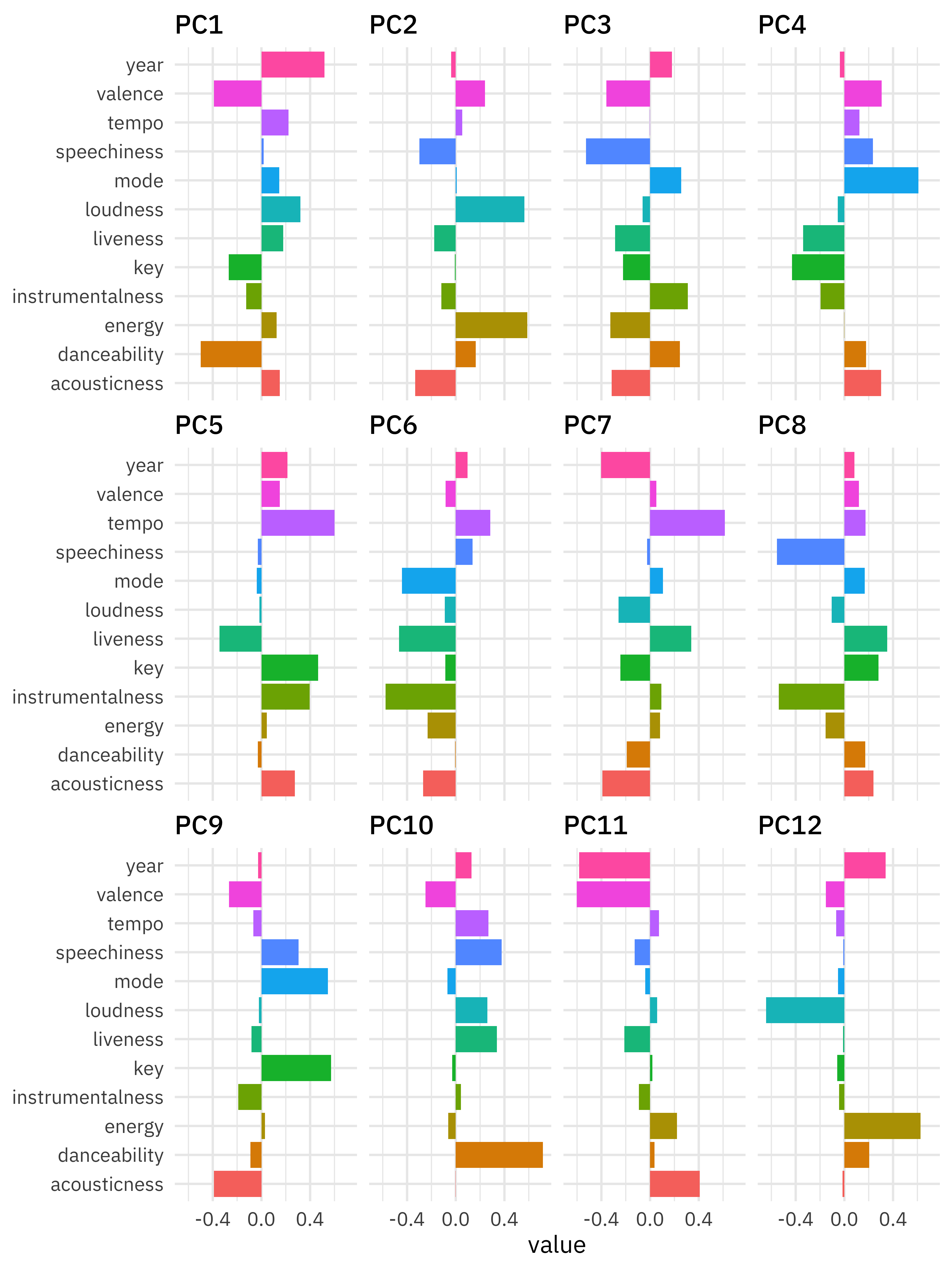
Once we have that done, we can both explore the results of the PCA and then eventually use it in a model. Let’s start with checking out how the PCA turned out. We can tidy() any of our recipe steps, including the PCA step, which is the third step. Then let’s make a visualization to see what the components look like.
tidied_pca <- tidy(ranking_prep, 3)

tidied_pca %>%
  mutate(component = fct_inorder(component)) %>%
  ggplot(aes(value, terms, fill = terms)) +
  geom_col(show.legend = FALSE) +
  facet_wrap(~component) +
  labs(y = NULL)
Let’s zoom in on the first four components.
library(tidytext)

tidied_pca %>%
  filter(component %in% c("PC1", "PC2", "PC3", "PC4")) %>%
  group_by(component) %>%
  top_n(6, abs(value)) %>%
  ungroup() %>%
  mutate(terms = reorder_within(terms, abs(value), component)) %>%
  ggplot(aes(abs(value), terms, fill = value > 0)) +
  geom_col() +
  facet_wrap(~component, scales = "free_y") +
  scale_y_reordered() +
  labs(
    x = "Absolute value of contribution",
    y = NULL, fill = "Positive?"
  )
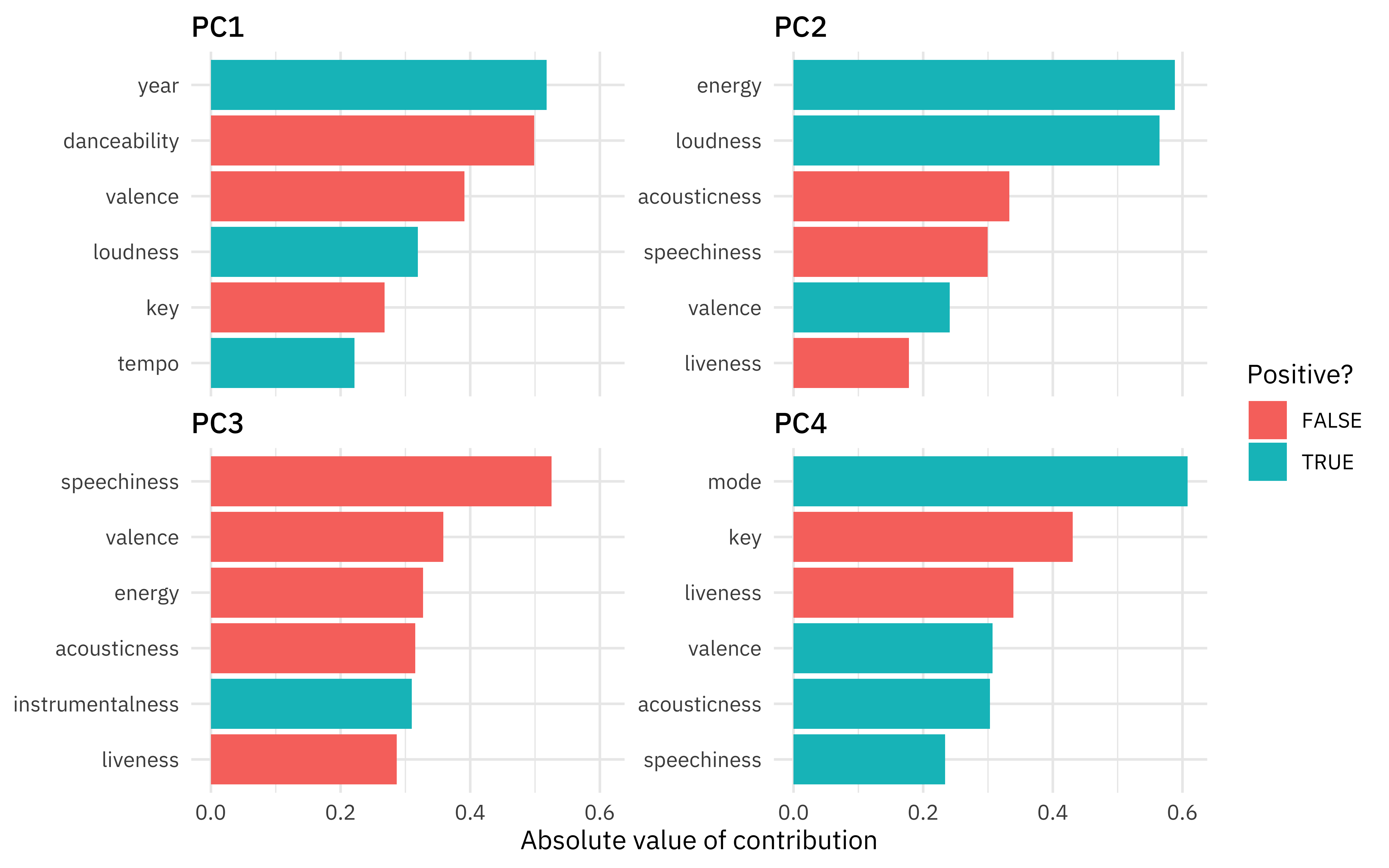
So PC1 is mostly about age and danceability, PC2 is mostly energy and loudness, PC3 is mostly speechiness, and PC4 is about the musical characteristics (actual key and major vs. minor key).
How are the songs distributed in the plane of the first two components?
juice(ranking_prep) %>%
  ggplot(aes(PC1, PC2, label = title)) +
  geom_point(alpha = 0.2) +
  geom_text(check_overlap = TRUE, family = "IBMPlexSans")
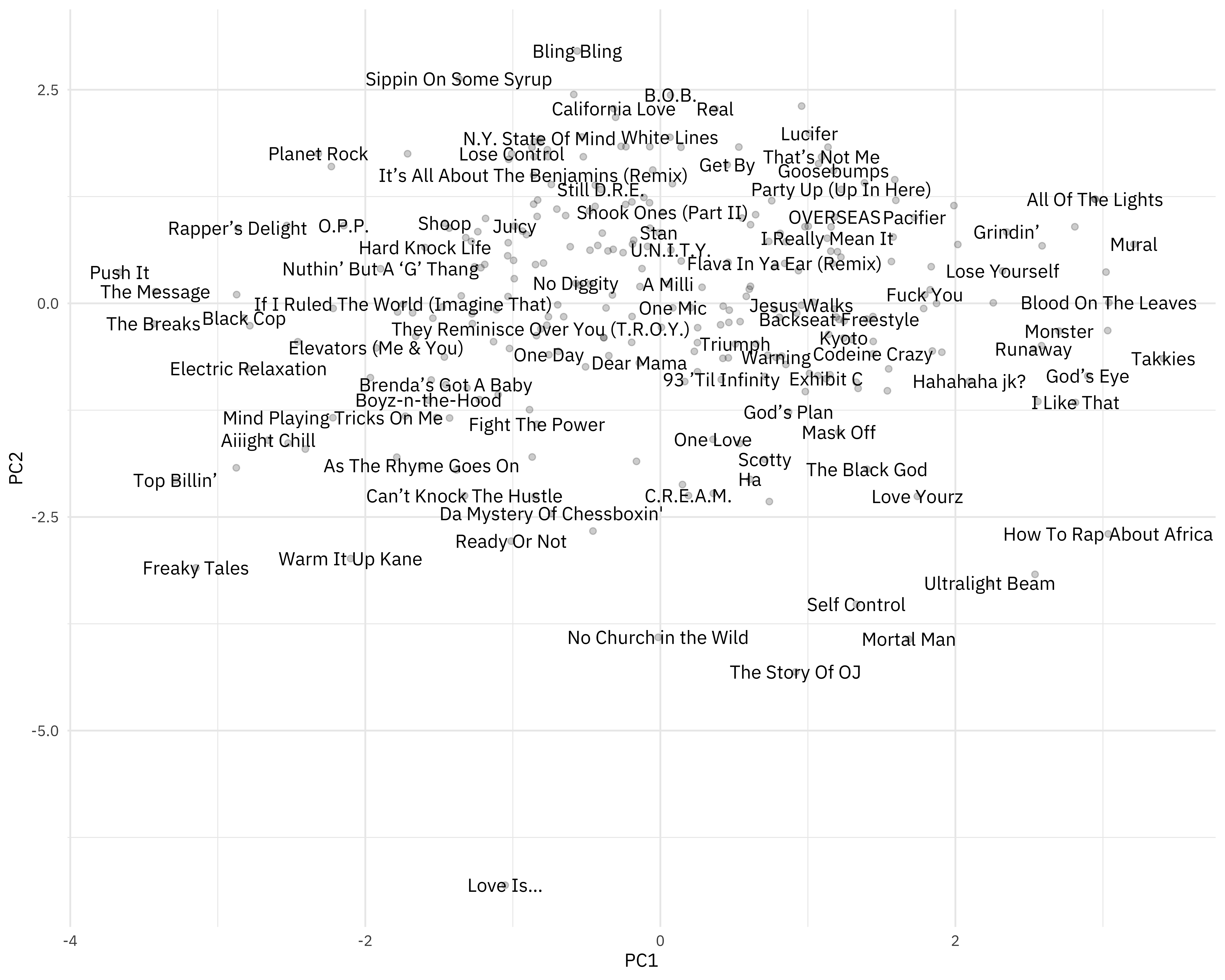
- Older, more danceable songs are to the left.
- Higher energy, louder songs are towards the top.
You can change out PC2 for PC3, for example, to instead see where more “speechy” songs are.
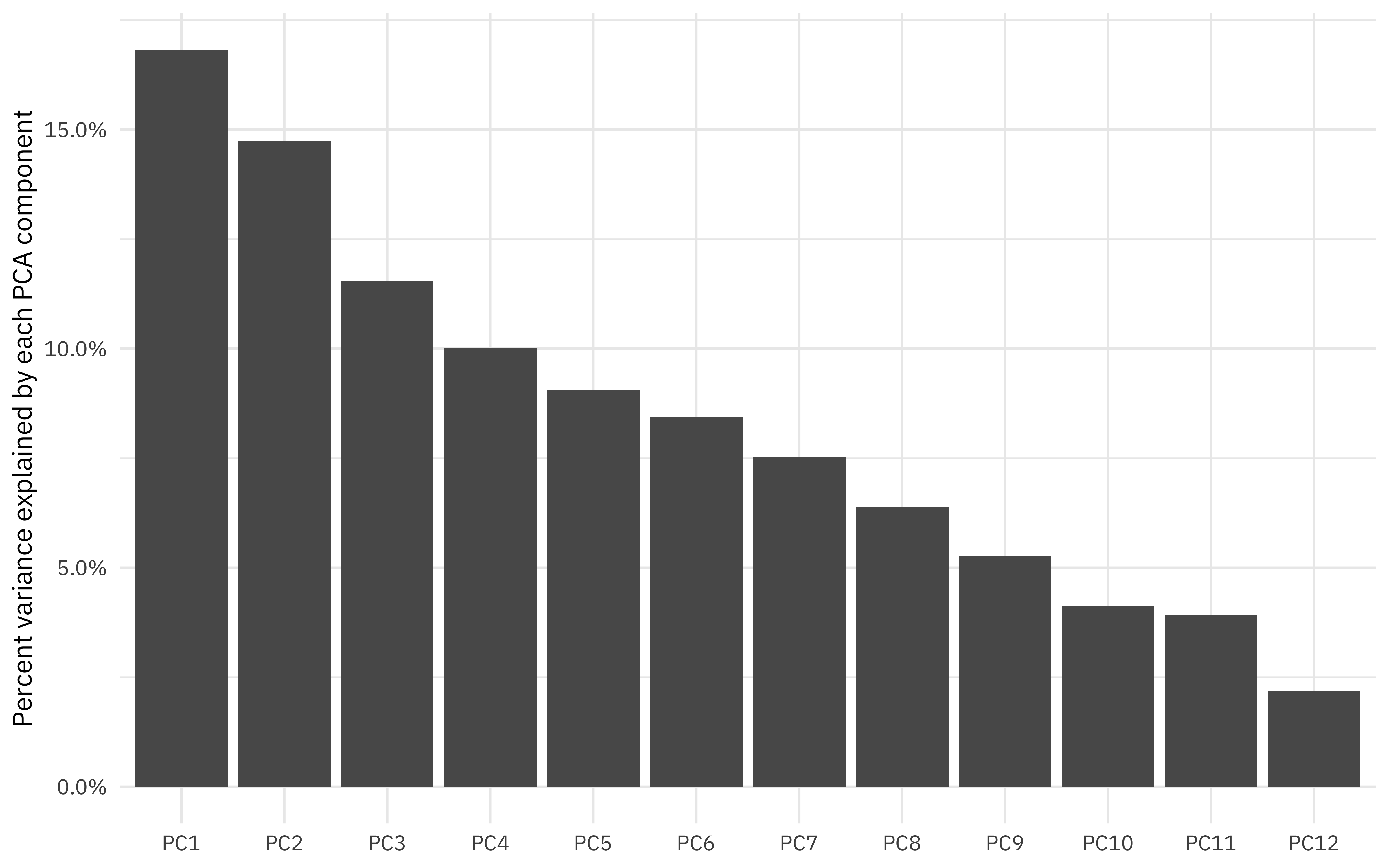
How much variation are we capturing?
sdev <- ranking_prep$steps[[3]]$res$sdev

percent_variation <- sdev^2 / sum(sdev^2)

tibble(
  component = unique(tidied_pca$component),
  percent_var = percent_variation ## use cumsum() to find cumulative, if you prefer
) %>%
  mutate(component = fct_inorder(component)) %>%
  ggplot(aes(component, percent_var)) +
  geom_col() +
  scale_y_continuous(labels = scales::percent_format()) +
  labs(x = NULL, y = "Percent variance explained by each PCA component")
And finally, let’s fit the same kind of model we fit before, but now with juice(ranking_prep). This approach really emphasizes how recipes can be used for data preprocessing. Notice how juice(ranking_prep) has already taken the log of points, has the component values ready to go, etc.
juice(ranking_prep)
## # A tibble: 293 x 8
##    title        artist             points     PC1    PC2     PC3    PC4      PC5
##    <fct>        <fct>               <dbl>   <dbl>  <dbl>   <dbl>  <dbl>    <dbl>
##  1 Juicy        The Notorious B.I…   4.94 -0.987   0.904 -1.10    1.16   5.46e-1
##  2 Fight The P… Public Enemy         4.61 -0.837  -1.42   0.686   0.184 -1.78e+0
##  3 Shook Ones … Mobb Deep            4.54  0.0153  1.06  -0.929   0.681 -3.27e-1
##  4 The Message  Grandmaster Flash…   4.50 -3.42    0.138 -0.0333 -0.653 -2.63e-4
##  5 Nuthin’ But… Dr Dre ft. Snoop …   4.43 -1.90    0.405 -0.629  -1.18   8.27e-2
##  6 C.R.E.A.M.   Wu-Tang Clan         4.13  0.190  -2.25  -1.94   -0.245  2.80e+0
##  7 93 ’Til Inf… Souls of Mischief    3.91  0.413  -0.892 -0.576   1.93   1.20e+0
##  8 Passin’ Me … The Pharcyde         3.87 -0.990   0.289 -0.607  -0.615 -1.01e+0
##  9 N.Y. State … Nas                  3.83 -0.819   1.93  -1.41   -0.736 -5.23e-1
## 10 Dear Mama    2Pac                 3.74 -0.143  -0.698  1.19    0.349 -4.05e-1
## # … with 283 more rows
pca_fit <- juice(ranking_prep) %>%
  select(-title, -artist) %>%
  lm(points ~ ., data = .)

summary(pca_fit)
##
## Call:
## lm(formula = points ~ ., data = .)
##
## Residuals:
##      Min       1Q   Median       3Q      Max
## -1.55257 -0.58620  0.04886  0.39583  2.89017
##
## Coefficients:
##             Estimate Std. Error t value Pr(>|t|)
## (Intercept)  1.92516    0.04944  38.936   <2e-16 ***
## PC1         -0.07547    0.03487  -2.165   0.0312 *
## PC2          0.03540    0.03725   0.950   0.3428
## PC3         -0.07129    0.04207  -1.695   0.0912 .
## PC4         -0.03100    0.04520  -0.686   0.4934
## PC5         -0.04195    0.04749  -0.883   0.3778
## ---
## Signif. codes:  0 '***' 0.001 '**' 0.01 '*' 0.05 '.' 0.1 ' ' 1
##
## Residual standard error: 0.8463 on 287 degrees of freedom
## Multiple R-squared:  0.03273,	Adjusted R-squared:  0.01588
## F-statistic: 1.942 on 5 and 287 DF,  p-value: 0.08738
So what did we find? There is some evidence here that older, more danceable, higher valence songs (PC1) were rated higher by critics.
- Posted on:
- April 14, 2020
- Length:
- 12 minute read, 2491 words
- Categories:
- rstats tidymodels
- Tags:
- rstats tidymodels