Classification metrics for #TidyTuesday GPT detectors

This is the latest in my series of screencasts! This screencast focuses on how to use tidymodels for computing classification metrics, using this week’s #TidyTuesday dataset on GPT detectors. 🤖

Here is the code I used in the video, for those who prefer reading instead of or in addition to video.

Explore data

We’re not going to train a model here, but instead use the output (i.e. predictions) from a handful of models that have been trained to detect text output from GPT. Let’s start by reading in the data:

library(tidyverse)
library(detectors)

detectors

## # A tibble: 6,185 × 9
##    kind  .pred_AI .pred_class detector     native name  model document_id prompt
##    <fct>    <dbl> <fct>       <chr>        <chr>  <chr> <chr>       <dbl> <chr> 
##  1 Human 1.00     AI          Sapling      No     Real… Human         497 <NA>  
##  2 Human 0.828    AI          Crossplag    No     Real… Human         278 <NA>  
##  3 Human 0.000214 Human       Crossplag    Yes    Real… Human         294 <NA>  
##  4 AI    0        Human       ZeroGPT      <NA>   Fake… GPT3          671 Plain 
##  5 AI    0.00178  Human       Originality… <NA>   Fake… GPT4          717 Eleva…
##  6 Human 0.000178 Human       HFOpenAI     Yes    Real… Human         855 <NA>  
##  7 AI    0.992    AI          HFOpenAI     <NA>   Fake… GPT3          533 Plain 
##  8 AI    0.0226   Human       Crossplag    <NA>   Fake… GPT4          484 Eleva…
##  9 Human 0        Human       ZeroGPT      Yes    Real… Human         781 <NA>  
## 10 Human 1.00     AI          Sapling      No     Real… Human         460 <NA>  
## # ℹ 6,175 more rows

The kind variable tells us whether a document was written by a human or generated via GPT, and the two .pred_* variables tells us what detector thought about that text, the predicted probability (.pred_AI) and predicted class (.pred_class) of that text being generated by AI. The native variable records whether a certain document was written by a native English writer or not.

detectors |> 
  count(native, kind, .pred_class)

## # A tibble: 6 × 4
##   native kind  .pred_class     n
##   <chr>  <fct> <fct>       <int>
## 1 No     Human AI            390
## 2 No     Human Human         247
## 3 Yes    Human AI             59
## 4 Yes    Human Human        1772
## 5 <NA>   AI    AI           1158
## 6 <NA>   AI    Human        2559

This is a great example for talking about classification metrics, because we are in a pretty common situation where a variable of interest (native) only applies to one class, the real humans. The AI-generated texts were certainly not generated by a native English writer, but they also were not generated by a non-native English writer.

For the real humans, what is the distribution of predicted probability for native and non-native English writers?

detectors |> 
  filter(!is.na(native)) |> 
  mutate(native = case_when(native == "Yes" ~ "Native English writer",
                            native == "No" ~ "Non-native English writer")) |> 
  ggplot(aes(.pred_AI, fill = native)) +
  geom_histogram(bins = 40, show.legend = FALSE) +
  facet_wrap(vars(native), scales = "free_y", nrow = 2) 

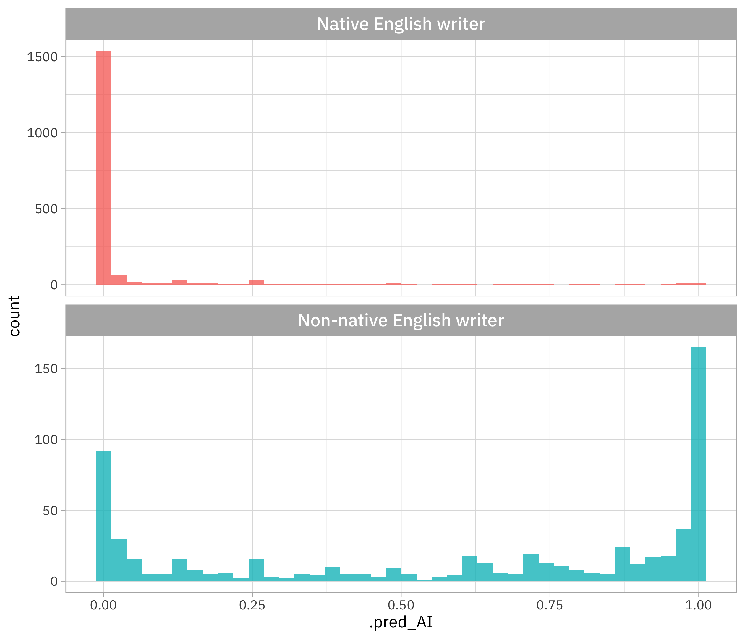
This is the main point of the paper this data comes from: GPT detectors are much more wrong for non-native English writers than for native writers. Pretty dramatic! Let’s walk through how to use classification metrics to measure this in a different way from looking at the distribution overall.

These GPT detectors are classification models (predicting “human” vs. “AI”), and there are two main categories of metrics for classification models:

• Metrics that use a predicted class, like “human” or “AI”
• Metrics that use a predicted probability, like .pred_AI = 0.828

Metrics that use a predicted class

In tidymodels, the package that handles model metrics is yardstick. Let’s start by making a confusion matrix, which uses the predicted classes, for the dataset as a whole:

library(yardstick)

detectors |> 
  conf_mat(kind, .pred_class)

##           Truth
## Prediction   AI Human
##      AI    1158   449
##      Human 2559  2019

This \(2 \times 2\) matrix or table tells us specifics about how these models are right and wrong. Overall, these models look to be better at identifying human documents (2019 right vs. 449 wrong) than identifying AI documents (1158 right vs. 2559 wrong).

One of the most common metrics for classification models is accuracy, just the plain old proportion of our data that is predicted correctly:

detectors |> 
  accuracy(kind, .pred_class)

## # A tibble: 1 × 3
##   .metric  .estimator .estimate
##   <chr>    <chr>          <dbl>
## 1 accuracy binary         0.514

Random guessing for a binary classification problem will give you 0.5, so here we see that these detectors are not much better than random guessing, aggregated over all these documents and different models/detectors. Do some detectors do better than others?

detectors |> 
  group_by(detector) |> 
  accuracy(kind, .pred_class)

## # A tibble: 7 × 4
##   detector      .metric  .estimator .estimate
##   <chr>         <chr>    <chr>          <dbl>
## 1 Crossplag     accuracy binary         0.501
## 2 GPTZero       accuracy binary         0.489
## 3 HFOpenAI      accuracy binary         0.514
## 4 OriginalityAI accuracy binary         0.590
## 5 Quil          accuracy binary         0.478
## 6 Sapling       accuracy binary         0.5  
## 7 ZeroGPT       accuracy binary         0.517

There is a little bit of variation here, I guess. What about differences across the native variable?

detectors |> 
  group_by(native) |> 
  accuracy(kind, .pred_class)

## # A tibble: 3 × 4
##   native .metric  .estimator .estimate
##   <chr>  <chr>    <chr>          <dbl>
## 1 No     accuracy binary         0.388
## 2 Yes    accuracy binary         0.968
## 3 <NA>   accuracy binary         0.312

This is now a much bigger difference. Notice that the accuracy for native English writers is GREAT while for non-native English writers it’s not much better than for the AI documents (remember that native = NA here means an AI generated document).

If you’ve learned a bit about ML, you probably have heard that accuracy is often not a great metric (especially when you have much class imbalance) so let’s try out a pair of related metrics that tell us the true positive rate and true negative rate.

Sensitivity tells us the true positive rate:

detectors |> 
  sensitivity(kind, .pred_class)

## # A tibble: 1 × 3
##   .metric     .estimator .estimate
##   <chr>       <chr>          <dbl>
## 1 sensitivity binary         0.312

detectors |> 
  group_by(detector) |> 
  sensitivity(kind, .pred_class)

## # A tibble: 7 × 4
##   detector      .metric     .estimator .estimate
##   <chr>         <chr>       <chr>          <dbl>
## 1 Crossplag     sensitivity binary         0.249
## 2 GPTZero       sensitivity binary         0.202
## 3 HFOpenAI      sensitivity binary         0.271
## 4 OriginalityAI sensitivity binary         0.444
## 5 Quil          sensitivity binary         0.379
## 6 Sapling       sensitivity binary         0.392
## 7 ZeroGPT       sensitivity binary         0.245

Sensitivity is a metric that can vary between 0 (bad) and 1 (good) so this looks like we will have lots of false negatives. Can we measure the true positive rate for different types of human writers?

detectors |> 
  group_by(native) |> 
  sensitivity(kind, .pred_class)

## # A tibble: 3 × 4
##   native .metric     .estimator .estimate
##   <chr>  <chr>       <chr>          <dbl>
## 1 No     sensitivity binary        NA    
## 2 Yes    sensitivity binary        NA    
## 3 <NA>   sensitivity binary         0.312

No, we can’t! Since there are no AI-generated documents written by native (or non-native) English writers, we can’t compute any metrics that need those empty elements of the confusion matrix:

detectors |> 
  filter(!is.na(native)) |> 
  conf_mat(kind, .pred_class)

##           Truth
## Prediction   AI Human
##      AI       0   449
##      Human    0  2019

Specificity, the true negative rate, works the same way, but “flipped”:

detectors |> 
  group_by(native) |> 
  specificity(kind, .pred_class)

## # A tibble: 3 × 4
##   native .metric     .estimator .estimate
##   <chr>  <chr>       <chr>          <dbl>
## 1 No     specificity binary         0.388
## 2 Yes    specificity binary         0.968
## 3 <NA>   specificity binary        NA

We can see that the true negative rate is much better for native English writers than non-native ones, but we can’t compute a true negative rate for only the AI-generated documents. This kind of situation comes up a fair amount for real models where a variable you are interested in only applies to one class in your classification problem.

Metrics that use a predicted probability

The other main category of metrics for this type of model use a probability rather than a class. If you have ever seen or used an ROC curve, it is an example of model evaluation that uses probabilities:

detectors |> 
    roc_curve(kind, .pred_AI) |> 
    autoplot()

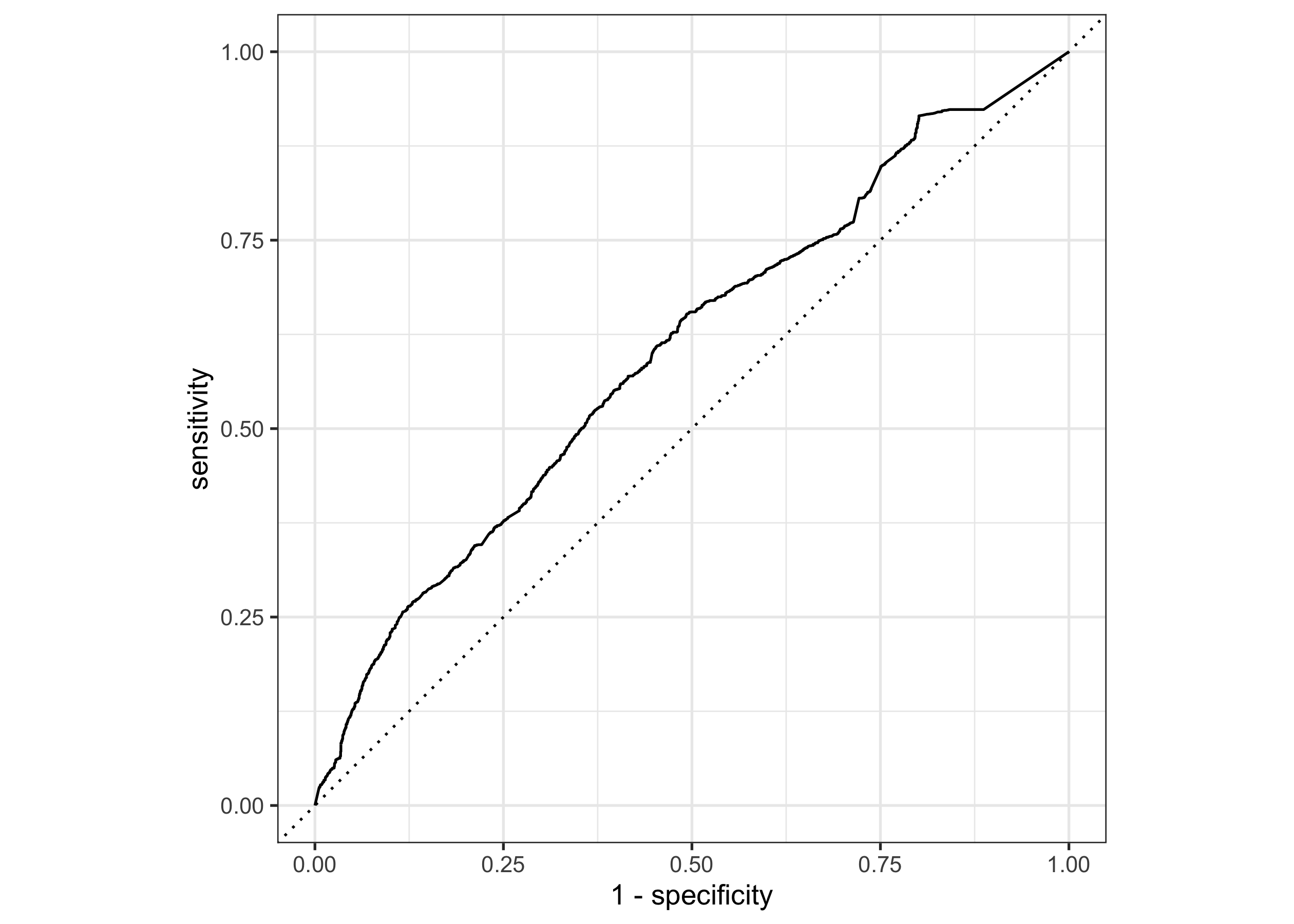
Notice how we’re using .pred_AI instead of .pred_class. How do the different detectors/models do in an ROC curve?

detectors |> 
    group_by(detector) |> 
    roc_curve(kind, .pred_AI) |> 
    autoplot()

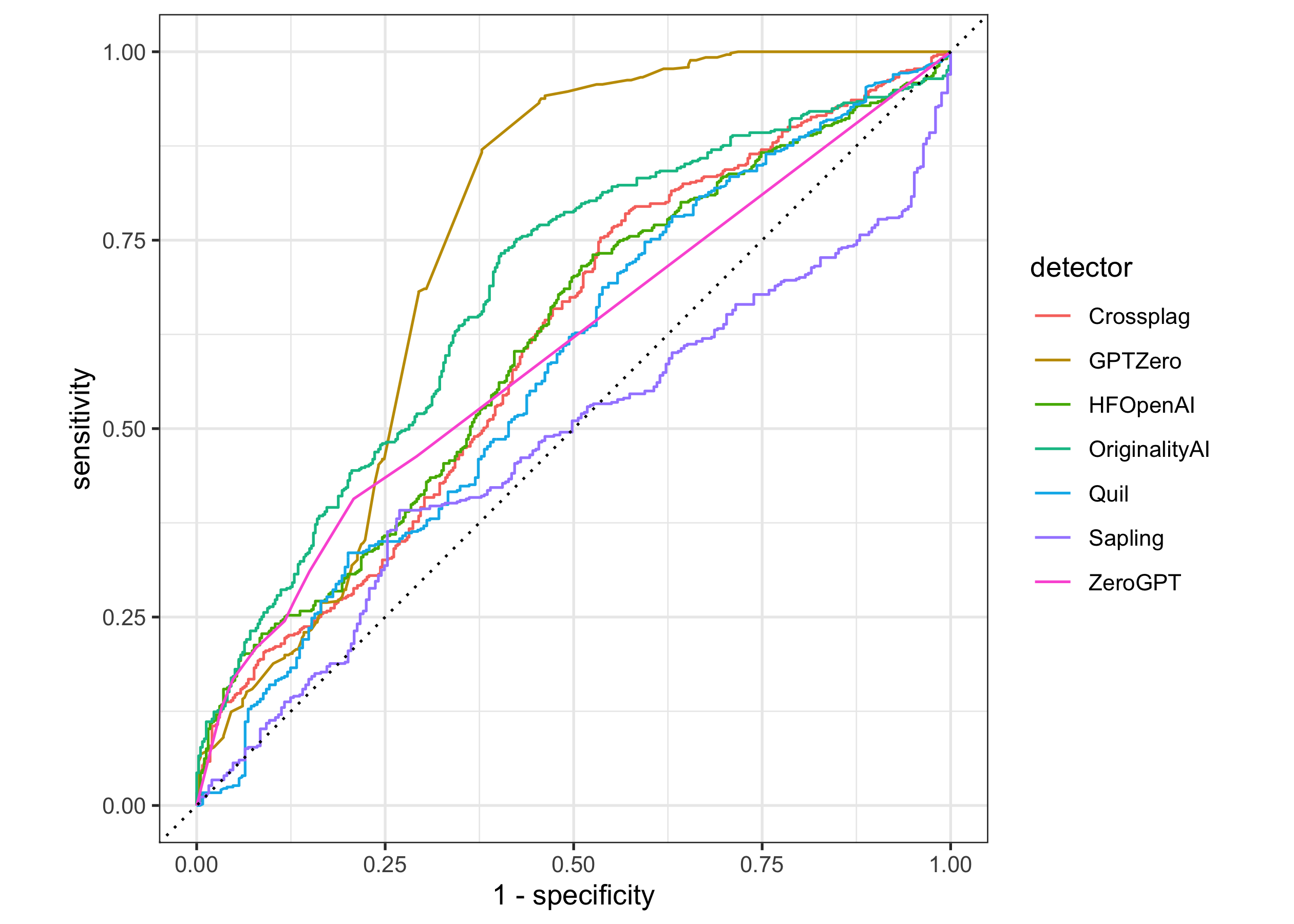
Yikes, OK. These curves can be used to compute the ROC AUC (area under the ROC curve):

detectors |> 
  group_by(detector) |> 
  roc_auc(kind, .pred_AI) 

## # A tibble: 7 × 4
##   detector      .metric .estimator .estimate
##   <chr>         <chr>   <chr>          <dbl>
## 1 Crossplag     roc_auc binary         0.613
## 2 GPTZero       roc_auc binary         0.750
## 3 HFOpenAI      roc_auc binary         0.614
## 4 OriginalityAI roc_auc binary         0.682
## 5 Quil          roc_auc binary         0.584
## 6 Sapling       roc_auc binary         0.480
## 7 ZeroGPT       roc_auc binary         0.603

Can we compute this kind of metric and compare across the native categories?

detectors |> 
    group_by(native) |> 
    roc_curve(kind, .pred_AI)

## Error in `roc_curve()`:
## ! No event observations were detected in `truth` with event level 'AI'.

Unfortunately, no, because in, say, the non-native English writer category, there are no AI-generated texts.

Let’s think about a metric that works in a different way, like mean log loss. This metric can distinguish between predictions that are a little wrong vs. very wrong; for example, it will say that a real human document with .pred_AI = 0.8 is predicted worse than one with .pred_AI = 0.6.

detectors |> 
    mn_log_loss(kind, .pred_AI)

## # A tibble: 1 × 3
##   .metric     .estimator .estimate
##   <chr>       <chr>          <dbl>
## 1 mn_log_loss binary          4.73

A log loss is better when it is lower. How does log loss vary over the detectors/models?

detectors |> 
    group_by(detector) |> 
    mn_log_loss(kind, .pred_AI) |> 
    arrange(.estimate)

## # A tibble: 7 × 4
##   detector      .metric     .estimator .estimate
##   <chr>         <chr>       <chr>          <dbl>
## 1 OriginalityAI mn_log_loss binary          1.94
## 2 Crossplag     mn_log_loss binary          2.81
## 3 HFOpenAI      mn_log_loss binary          2.83
## 4 Quil          mn_log_loss binary          3.18
## 5 GPTZero       mn_log_loss binary          4.60
## 6 Sapling       mn_log_loss binary          5.82
## 7 ZeroGPT       mn_log_loss binary         11.9

This is a pretty dramatic range in log loss. 😳 What about across the native variable?

detectors |> 
    group_by(native) |> 
    mn_log_loss(kind, .pred_AI)

## # A tibble: 3 × 4
##   native .metric     .estimator .estimate
##   <chr>  <chr>       <chr>          <dbl>
## 1 No     mn_log_loss binary         3.60 
## 2 Yes    mn_log_loss binary         0.116
## 3 <NA>   mn_log_loss binary         7.21

Here we see that the documents written by non-native English writers are predicted better than the AI-generated documents, but way, way worse than those by native Engish writers.