What tokens are used more vs. less in #TidyTuesday place names?

This is the latest in my series of screencasts! This screencast focuses on how to use tidymodels to learn a subword tokenization strategy, using this week’s #TidyTuesday dataset on place names in the United States. 🏞️

Here is the code I used in the video, for those who prefer reading instead of or in addition to video.

Explore data

Our modeling goal in this case is to predict the number of uses of geographical place names in the United States, to find out which kinds of names are more and less common. Let’s start by reading in the data:

library(tidyverse)

us_place_names <- read_csv('https://raw.githubusercontent.com/rfordatascience/tidytuesday/master/data/2023/2023-06-27/us_place_names.csv')

glimpse(us_place_names)

## Rows: 187,519
## Columns: 9
## $ feature_id     <dbl> 479, 492, 511, 538, 542, 580, 581, 605, 728, 765, 770, …
## $ feature_name   <chr> "Adamana", "Adobe", "Agua Fria", "Ajo", "Ak Chin", "Alh…
## $ state_name     <chr> "Arizona", "Arizona", "Arizona", "Arizona", "Arizona", …
## $ county_name    <chr> "Apache", "Maricopa", "Maricopa", "Pima", "Pinal", "Mar…
## $ county_numeric <dbl> 1, 13, 13, 19, 21, 13, 19, 13, 3, 21, 21, 25, 13, 17, 2…
## $ date_created   <date> 1980-02-08, 1980-02-08, 1980-02-08, 1980-02-08, 1980-0…
## $ date_edited    <date> 2022-06-07, 2022-06-07, 2022-06-07, 2022-06-07, 2022-0…
## $ prim_lat_dec   <dbl> 34.97669, 33.68921, 33.60559, 32.37172, 33.03283, 33.49…
## $ prim_long_dec  <dbl> -109.8223, -112.1227, -112.3146, -112.8607, -112.0732, …

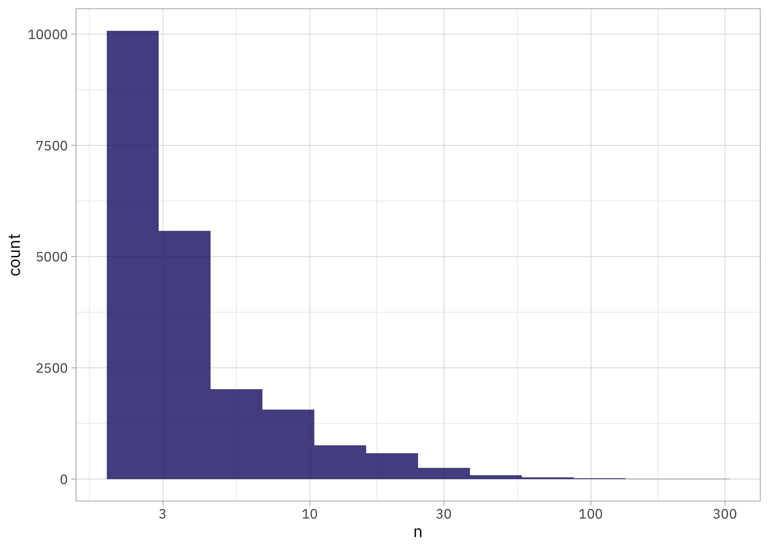
How many times is each place name used? Let’s restrict our analysis to place names used more than one time.

place_counts <- 
  us_place_names |> 
  count(feature_name, sort = TRUE) |> 
  filter(n > 1)

place_counts

## # A tibble: 20,974 × 2
##    feature_name       n
##    <chr>          <int>
##  1 Midway           215
##  2 Fairview         210
##  3 Oak Grove        169
##  4 Five Points      149
##  5 Riverside        127
##  6 Pleasant Hill    123
##  7 Mount Pleasant   119
##  8 Bethel           108
##  9 Centerville      107
## 10 New Hope         105
## # ℹ 20,964 more rows

So many Midways and Fairviews! As is common with text data, we see something like Zipf’s law:

place_counts |> 
  ggplot(aes(n)) +
  geom_histogram(bins = 12) +
  scale_x_log10()

Build a model

We can start by loading the tidymodels metapackage and splitting our data into training and testing sets. We don’t have much resampling to do in this analysis (and might not even really use the test set for much) but still think about this stage as spending your data budget.

library(tidymodels)

set.seed(123)
place_split <- initial_split(place_counts, strata = n)
place_train <- training(place_split)
place_test <- testing(place_split)

Next, let’s create our feature engineering recipe. Let’s tokenize using byte pair encoding; this is an algorithm that iteratively merges frequently occurring subword pairs and gets us information in between the character level and the word level. You can read more about byte pair encoding in this section of Supervised Machine Learning for Text Analysis in R. Byte pair encoding is used in LLMs like GPT models and friends, and it is great to understand how it works.

It would probably be a good idea to tune the vocabulary size using our text data to find the optimal value, but let’s just stick with a small-to-medium vocabulary for this dataset of place

library(textrecipes)

place_rec <- recipe(n ~ feature_name, data = place_train) |> 
  step_tokenize_bpe(feature_name, vocabulary_size = 200) |>
  step_tokenfilter(feature_name, max_tokens = 100) |>
  step_tf(feature_name)

place_rec

There are a number of specialized packages, outside the core tidymodels packages, for less general, more specialized data analysis and modeling tasks. One of these is poissonreg, for Poisson regression models such as those we can use with this count data. The counts here are the number of times each place name is used. Since we aren’t tuning anything, we can just go ahead and fit our model to our training data.

library(poissonreg)
poisson_wf <- workflow(place_rec, poisson_reg())
poisson_fit <- fit(poisson_wf, place_train)

Understand our model results

We can tidy() our fitted model to get out the coefficients. What are the top 20 subwords that drive the number of uses in US place names either up or down?

tidy(poisson_fit) |> 
  filter(term != "(Intercept)") |> 
  mutate(term = str_remove_all(term, "tf_feature_name_")) |> 
  slice_max(abs(estimate), n = 20) |> 
  arrange(-estimate)

## # A tibble: 20 × 5
##    term            estimate std.error statistic   p.value
##    <chr>              <dbl>     <dbl>     <dbl>     <dbl>
##  1 wood               0.310    0.0223     13.9  6.71e- 44
##  2 id                 0.258    0.0266      9.68 3.81e- 22
##  3 `▁L`              -0.228    0.0180    -12.7  8.66e- 37
##  4 `▁R`              -0.238    0.0183    -13.0  1.49e- 38
##  5 ou                -0.244    0.0360     -6.80 1.07e- 11
##  6 et                -0.252    0.0321     -7.87 3.51e- 15
##  7 `▁Br`             -0.258    0.0280     -9.23 2.70e- 20
##  8 `▁B`              -0.259    0.0170    -15.2  2.63e- 52
##  9 `▁Park`           -0.260    0.0258    -10.1  8.28e- 24
## 10 at                -0.281    0.0245    -11.5  2.03e- 30
## 11 `▁D`              -0.282    0.0218    -12.9  3.75e- 38
## 12 `▁Co`             -0.285    0.0264    -10.8  4.86e- 27
## 13 ill               -0.296    0.0322     -9.19 3.89e- 20
## 14 ac                -0.320    0.0260    -12.3  6.94e- 35
## 15 `▁T`              -0.352    0.0212    -16.6  9.17e- 62
## 16 `▁K`              -0.361    0.0288    -12.5  6.12e- 36
## 17 es                -0.423    0.0253    -16.7  8.98e- 63
## 18 `▁Heights`        -0.497    0.0318    -15.6  4.53e- 55
## 19 `▁Estates`        -0.573    0.0306    -18.8  1.91e- 78
## 20 `▁(historical)`   -0.621    0.0175    -35.5  2.78e-276

Looks like there are lots of place names that include “wood”, and subwords like “historical”, “Estates”, and “Heights” are less common. What are some of these names like?

place_train |> 
  filter(str_detect(feature_name, "Estates|wood"))

## # A tibble: 640 × 2
##    feature_name           n
##    <chr>              <int>
##  1 Allwood                3
##  2 Basswood               3
##  3 Bear Creek Estates     3
##  4 Belair Estates         3
##  5 Belmont Estates        3
##  6 Bingham Estates        3
##  7 Birchwood Estates      3
##  8 Boulevard Estates      3
##  9 Braddock Estates       3
## 10 Brandywine Estates     3
## # ℹ 630 more rows

Let’s make a visualization.

place_train |> 
  filter(str_detect(feature_name, "Estates|wood")) |> 
  mutate(feature_name = case_when(
    str_detect(feature_name, "wood") ~ "wood",
    str_detect(feature_name, "Estates") ~ "estate"
  )) |> 
  ggplot(aes(n, fill = feature_name)) +
  geom_histogram(alpha = 0.8, position = "dodge", bins = 12) +
  scale_x_log10() +
  labs(x = "Number of place name uses",
       y = "Count",
       fill = NULL)

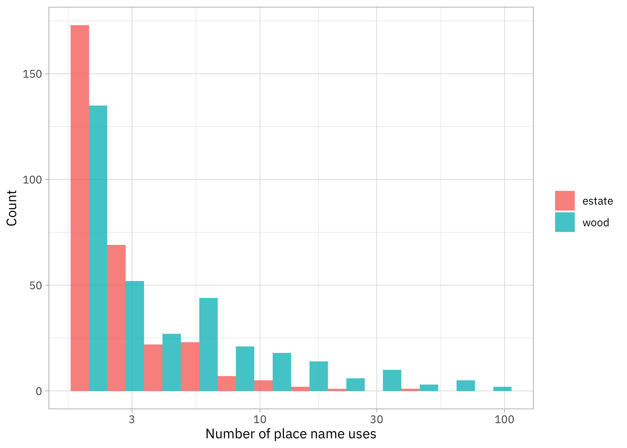
In this dataset of place names in the US, woods are more numerous, while estates are less numerous.

We didn’t train this model with an eye to predictive performance, but it’s often still a good idea to estimate how well a model fits the data using an appropriate model metric. Since we are predicting counts, we can use a metric appropriate for count data like poisson_log_loss(), and as always, we do not estimate performance using the same data we trained with, but rather the test data:

augment(poisson_fit, place_test) |> 
  poisson_log_loss(n, .pred)

## # A tibble: 1 × 3
##   .metric          .estimator .estimate
##   <chr>            <chr>          <dbl>
## 1 poisson_log_loss standard        3.53

If we wanted to tune the vocabulary_size for the byte pair encoding tokenization, we would use a metric appropriate for this problem like poisson_log_loss(). For more on using Poisson regression, check out Chapter 21 of Tidy Modeling with R.