Which #TidyTuesday post offices are in Hawaii?
By Julia Silge in rstats tidymodels
April 14, 2021
This is the latest in my series of
screencasts demonstrating how to use the
tidymodels packages, from starting out with first modeling steps to tuning more complex models. Today’s screencast walks through how to use text information at the subword level in predictive modeling, with this week’s
#TidyTuesday dataset on United States post offices. 📬
Here is the code I used in the video, for those who prefer reading instead of or in addition to video.
Explore data
Our modeling goal is to predict whether a post office is in Hawaii or not based on the name of the office in this week’s #TidyTuesday dataset.
Let’s start by reading in the data.
library(tidyverse)

post_offices <- read_csv("https://raw.githubusercontent.com/rfordatascience/tidytuesday/master/data/2021/2021-04-13/post_offices.csv")
How many post offices are there in each state?
post_offices %>%
  count(state, sort = TRUE)
## # A tibble: 53 x 2
##    state     n
##    <chr> <int>
##  1 PA     8534
##  2 TX     7772
##  3 KY     7432
##  4 VA     7085
##  5 NC     6547
##  6 MO     6232
##  7 NY     6111
##  8 TN     6025
##  9 GA     5754
## 10 OH     5537
## # … with 43 more rows
In Hawaii, the names of the post offices are unique, but there are not many at all, compared to the other states.
post_offices %>%
  filter(state == "HI") %>%
  pull(name)
##   [1] "AIEA"                 "ANAHOLA"              "CANTON ISLAND"
##   [4] "CAPTAIN COOK"         "COCONUT ISLAND"       "ELEELE"
##   [7] "EWA"                  "EWA BEACH"            "FERNDALE"
##  [10] "FORT KAMEHAMEHA"      "FORT SHAFTER"         "GLENWOOD"
##  [13] "HAIKU"                "HAINA"                "HAIULA"
##  [16] "HAKALAU"              "HALAULA"              "HALAWA"
##  [19] "HALEIWA"              "HALEIWA"              "HALIIMAILE RURAL BR."
##  [22] "HAMAKUA"              "HAMAKUAPOKO"          "HAMOA"
##  [25] "HANA"                 "HANALEI"              "HANAMAULU"
##  [28] "HANAPEPE"             "HATANLA"              "HAUULA"
##  [31] "HAUULA"               "HAWAII NATIONAL PARK" "HAWI"
##  [34] "HEEIA"                "HICKAM FIELD BR."     "HILEA"
##  [37] "HILO"                 "HOLUALOA"             "HOMESTEAD"
##  [40] "HONALUA"              "HONAUNAU"             "HONOKAA"
##  [43] "HONOKOHAU"            "HONOKOHUA"            "HONOLUA"
##  [46] "HONOLULU"             "HONOMU"               "HONOULIULI"
##  [49] "HONUAPO"              "HOOKENA"              "HOOLEHUA"
##  [52] "HOOPULOA"             "HUEHUE"               "HUELO"
##  [55] "KAAAWA"               "KAALAEA"              "KAANAPALI"
##  [58] "KAHAKULOA"            "KAHANA"               "KAHUKU"
##  [61] "KAHULUI"              "KAI MALINO"           "KAILUA"
##  [64] "KAILUA KONA"          "KALAE"                "KALAHEO"
##  [67] "KALAPANA"             "KALAPANA"             "KALAUPAPA"
##  [70] "KALAWAO"              "KALOA"                "KAMALO"
##  [73] "KAMUELA"              "KANEOHE"              "KAPAA"
##  [76] "KAPAA"                "KAPAAU"               "KAPOHO"
##  [79] "KAPOLEI"              "KAULAWAI"             "KAUMAKANI"
##  [82] "KAUNAKAKAI"           "KAUPO"                "KAWAIHAE"
##  [85] "KAWAILOA"             "KEAAU"                "KEAAU"
##  [88] "KEAHUA"               "KEALAKEKUA"           "KEALIA"
##  [91] "KEANAE"               "KEAUHOU"              "KEKAHA"
##  [94] "KEOKEA"               "KEOMUKU"              "KIHEI"
##  [97] "KILAUEA"              "KIPAHULU"             "KOHALA"
## [100] "KOLOA"                "KONA"                 "KUALAPUU"
## [103] "KUKUAIAU"             "KUKUIHAELE"           "KUNIA"
## [106] "KURTISTOWN"           "LAHAINA"              "LAIE"
## [109] "LALAMILO"             "LANAI CITY"           "LANIKAI"
## [112] "LAUPAHOEHOE"          "LAWAI"                "LIBBYVILLE"
## [115] "LIHUE"                "LUKE FIELD BR."       "MAHUKONA"
## [118] "MAKAWAO"              "MAKAWELI"             "MAKENA"
## [121] "MAKUA"                "MANA"                 "MAUNA LOA"
## [124] "MAUNALOA"             "MAUNAWEI"             "MIDWAY ISLAND"
## [127] "MOUNTAINVIEW"         "NAALEHU"              "NAHIKU"
## [130] "NAHIKU"               "NANAKULI"             "NANAKULI"
## [133] "NAPOOPOO"             "NINOLE"               "OLAA"
## [136] "OLLA PLANTATION"      "OLOWALU"              "OOKALA"
## [139] "OPIHIKAO"             "PAAUHAU"              "PAAUILO"
## [142] "PAHALA"               "PAHOA"                "PAIA"
## [145] "PAPAALOA"             "PAPAIKOU"             "PAPAIKOU"
## [148] "PAUWELA"              "PEAHI"                "PEARL CITY"
## [151] "PEARL HARBOR"         "PEARL HARBOR"         "PELEKUNU"
## [154] "PEPEEKEO"             "POHOKI"               "PRINCEVILLE"
## [157] "PUHI"                 "PUKALANI"             "PUKOO"
## [160] "PUKOO"                "PUNALUU"              "PUULOA HALE BR."
## [163] "PUUNENE"              "ROOSEVELT"            "SCHOFIELD BARRACKS"
## [166] "SPRECKELSVILLE"       "SPRECKELSVILLE"       "SUNSET BEACH"
## [169] "ULUPALAKUA"           "ULUPALAKUA"           "VOLCANO"
## [172] "VOLCANO HOUSE"        "WAHIAWA"              "WAIAHOLE"
## [175] "WAIAKOA"              "WAIALEE"              "WAIALUA"
## [178] "WAIANAE"              "WAIHEE"               "WAIHEE"
## [181] "WAIKANE"              "WAIKAUPU"             "WAIKOLOA"
## [184] "WAILUKU"              "WAIMANALO"            "WAIMEA"
## [187] "WAIMEA"               "WAINIHA"              "WAIOHINU"
## [190] "WAIPAHU"              "WAIPIO"               "WATERTOWN"
Build a model
We can start by loading the tidymodels metapackage, splitting our data into training and testing sets, and creating cross-validation samples. Think about this stage as spending your data budget.
library(tidymodels)

set.seed(123)
po_split <- post_offices %>%
  mutate(state = case_when(
    state == "HI" ~ "Hawaii",
    TRUE ~ "Other"
  )) %>%
  select(name, state) %>%
  initial_split(strate = state)

po_train <- training(po_split)
po_test <- testing(po_split)

set.seed(234)
po_folds <- vfold_cv(po_train, strata = state)
po_folds
## #  10-fold cross-validation using stratification
## # A tibble: 10 x 2
##    splits                 id
##    <list>                 <chr>
##  1 <split [112144/12461]> Fold01
##  2 <split [112144/12461]> Fold02
##  3 <split [112144/12461]> Fold03
##  4 <split [112144/12461]> Fold04
##  5 <split [112144/12461]> Fold05
##  6 <split [112145/12460]> Fold06
##  7 <split [112145/12460]> Fold07
##  8 <split [112145/12460]> Fold08
##  9 <split [112145/12460]> Fold09
## 10 <split [112145/12460]> Fold10
Next, let’s create our feature engineering recipe. Let’s tokenize using byte pair encoding; this is an algorithm that iteratively merges frequently occurring subword pairs and gets us information in between character-level and word-level. You can read more about byte pair encoding in this section of Supervised Machine Learning for Text Analysis in R.
library(textrecipes)
library(themis)

po_rec <- recipe(state ~ name, data = po_train) %>%
  step_tokenize(name,
    engine = "tokenizers.bpe",
    training_options = list(vocab_size = 200)
  ) %>%
  step_tokenfilter(name, max_tokens = 200) %>%
  step_tf(name) %>%
  step_normalize(all_predictors()) %>%
  step_smote(state)

po_rec
## Data Recipe
##
## Inputs:
##
##       role #variables
##    outcome          1
##  predictor          1
##
## Operations:
##
## Tokenization for name
## Text filtering for name
## Term frequency with name
## Centering and scaling for all_predictors()
## SMOTE based on state
We also are upsampling this very imbalanced data set via step_smote() from the
themis package. The results of this data preprocessing show us the subword features.
po_rec %>%
  prep() %>%
  bake(new_data = NULL)
## # A tibble: 248,932 x 201
##    `tf_name_-` tf_name_. `tf_name_'` `tf_name_'S` `tf_name_/` `tf_name_&`
##          <dbl>     <dbl>       <dbl>        <dbl>       <dbl>       <dbl>
##  1     -0.0203   -0.0184     -0.0346       -0.165     -0.0102    -0.00567
##  2     -0.0203  102.         -0.0346       -0.165     -0.0102    -0.00567
##  3     -0.0203   -0.0184     -0.0346       -0.165     -0.0102    -0.00567
##  4     -0.0203   -0.0184     -0.0346       -0.165     -0.0102    -0.00567
##  5     -0.0203   -0.0184     -0.0346       -0.165     -0.0102    -0.00567
##  6     -0.0203   -0.0184     -0.0346       -0.165     -0.0102    -0.00567
##  7     -0.0203   -0.0184     -0.0346       -0.165     -0.0102    -0.00567
##  8     -0.0203   -0.0184     -0.0346       -0.165     -0.0102    -0.00567
##  9     -0.0203   -0.0184     -0.0346       -0.165     -0.0102    -0.00567
## 10     -0.0203   -0.0184     -0.0346       -0.165     -0.0102    -0.00567
## # … with 248,922 more rows, and 195 more variables: tf_name_` <dbl>,
## #   tf_name_▁ <dbl>, tf_name_▁A <dbl>, tf_name_▁AL <dbl>, tf_name_▁B <dbl>,
## #   tf_name_▁BE <dbl>, tf_name_▁BL <dbl>, tf_name_▁BR <dbl>, tf_name_▁C <dbl>,
## #   tf_name_▁CENT <dbl>, tf_name_▁CH <dbl>, tf_name_▁CITY <dbl>,
## #   tf_name_▁CL <dbl>, tf_name_▁CO <dbl>, tf_name_▁CREEK <dbl>,
## #   tf_name_▁D <dbl>, tf_name_▁E <dbl>, tf_name_▁EL <dbl>, tf_name_▁F <dbl>,
## #   tf_name_▁G <dbl>, tf_name_▁GRO <dbl>, tf_name_▁GROVE <dbl>,
## #   tf_name_▁H <dbl>, tf_name_▁HILL <dbl>, tf_name_▁J <dbl>, tf_name_▁K <dbl>,
## #   tf_name_▁L <dbl>, tf_name_▁LAKE <dbl>, tf_name_▁LE <dbl>, tf_name_▁M <dbl>,
## #   tf_name_▁MILL <dbl>, tf_name_▁MILLS <dbl>, tf_name_▁MO <dbl>,
## #   tf_name_▁MOUNT <dbl>, tf_name_▁N <dbl>, tf_name_▁NEW <dbl>,
## #   tf_name_▁NOR <dbl>, tf_name_▁O <dbl>, tf_name_▁P <dbl>, tf_name_▁PO <dbl>,
## #   tf_name_▁R <dbl>, tf_name_▁RI <dbl>, tf_name_▁RO <dbl>, tf_name_▁S <dbl>,
## #   tf_name_▁SH <dbl>, tf_name_▁SP <dbl>, tf_name_▁SPRING <dbl>,
## #   tf_name_▁SPRINGS <dbl>, tf_name_▁ST <dbl>, tf_name_▁T <dbl>,
## #   tf_name_▁V <dbl>, tf_name_▁W <dbl>, tf_name_▁WEST <dbl>, tf_name_▁WH <dbl>,
## #   tf_name_1 <dbl>, tf_name_A <dbl>, tf_name_AD <dbl>, tf_name_AG <dbl>,
## #   tf_name_AK <dbl>, tf_name_AKE <dbl>, tf_name_AL <dbl>, tf_name_ALE <dbl>,
## #   tf_name_ALL <dbl>, tf_name_AM <dbl>, tf_name_AN <dbl>, tf_name_AND <dbl>,
## #   tf_name_ANT <dbl>, tf_name_AP <dbl>, tf_name_AR <dbl>, tf_name_ARD <dbl>,
## #   tf_name_ARK <dbl>, tf_name_ART <dbl>, tf_name_AS <dbl>, tf_name_AST <dbl>,
## #   tf_name_AT <dbl>, tf_name_ATION <dbl>, tf_name_AW <dbl>, tf_name_AY <dbl>,
## #   tf_name_B <dbl>, tf_name_BER <dbl>, tf_name_BUR <dbl>, tf_name_BURG <dbl>,
## #   tf_name_C <dbl>, tf_name_CE <dbl>, tf_name_CH <dbl>, tf_name_CK <dbl>,
## #   tf_name_CO <dbl>, tf_name_D <dbl>, tf_name_E <dbl>, tf_name_ED <dbl>,
## #   tf_name_EE <dbl>, tf_name_EL <dbl>, tf_name_ELD <dbl>, tf_name_ELL <dbl>,
## #   tf_name_EN <dbl>, tf_name_ENT <dbl>, tf_name_ER <dbl>, tf_name_ERS <dbl>,
## #   tf_name_ES <dbl>, tf_name_EST <dbl>, …
Next let’s create a model specification for a linear support vector machine. This is a newer model in parsnip, currently in the development version on GitHub. Linear SVMs are often a good starting choice for text models.
svm_spec <- svm_linear() %>%
  set_mode("classification") %>%
  set_engine("LiblineaR")

svm_spec
## Linear Support Vector Machine Specification (classification)
##
## Computational engine: LiblineaR
Let’s put these together in a workflow.
po_wf <- workflow() %>%
  add_recipe(po_rec) %>%
  add_model(svm_spec)

po_wf
## ══ Workflow ════════════════════════════════════════════════════════════════════
## Preprocessor: Recipe
## Model: svm_linear()
##
## ── Preprocessor ────────────────────────────────────────────────────────────────
## 5 Recipe Steps
##
## ● step_tokenize()
## ● step_tokenfilter()
## ● step_tf()
## ● step_normalize()
## ● step_smote()
##
## ── Model ───────────────────────────────────────────────────────────────────────
## Linear Support Vector Machine Specification (classification)
##
## Computational engine: LiblineaR
Now let’s fit this workflow (that combines feature engineering with the SVM model) to the resamples we created earlier. The linear SVM model does not support class probabilities, so we need to set a custom metric_set() that only includes metrics for hard clss probabilities.
set.seed(234)

doParallel::registerDoParallel()
po_rs <- fit_resamples(
  po_wf,
  po_folds,
  metrics = metric_set(accuracy, sens, spec)
)
How did we do?
collect_metrics(po_rs)
## # A tibble: 3 x 6
##   .metric  .estimator  mean     n  std_err .config
##   <chr>    <chr>      <dbl> <int>    <dbl> <chr>
## 1 accuracy binary     0.971    10 0.000763 Preprocessor1_Model1
## 2 sens     binary     0.755    10 0.0386   Preprocessor1_Model1
## 3 spec     binary     0.972    10 0.000791 Preprocessor1_Model1
Not too bad, although you can tell we are doing better on one class than the other.
Fit and evaluate final model
Next, let’s fit our model on last time to the whole training set at once (rather than resampled data) and evaluate on the testing set. This is the first time we have touched the testing set.
final_fitted <- last_fit(
  po_wf,
  po_split,
  metrics = metric_set(accuracy, sens, spec)
)
collect_metrics(final_fitted)
## # A tibble: 3 x 4
##   .metric  .estimator .estimate .config
##   <chr>    <chr>          <dbl> <chr>
## 1 accuracy binary         0.969 Preprocessor1_Model1
## 2 sens     binary         0.811 Preprocessor1_Model1
## 3 spec     binary         0.969 Preprocessor1_Model1
Our performance on the testing set is about the same as what we found with our resampled data, which is good.
We can explore how the model is doing for both the positive and negative classes with a confusion matrix.
collect_predictions(final_fitted) %>%
  conf_mat(state, .pred_class)
##           Truth
## Prediction Hawaii Other
##     Hawaii     43  1273
##     Other      10 40209
This just really emphasizes what an imbalanced problem this is, but we can see how well we are doing for the post offices in Hawaii vs. the rest of the country.
We are still in the process of building out support for exploring results for the LiblineaR model (like a tidy() method) but in the meantime, you can get out the linear coefficients manually.
po_fit <- pull_workflow_fit(final_fitted$.workflow[[1]])
liblinear_obj <- po_fit$fit$W
liblinear_df <- tibble(
  term = colnames(liblinear_obj),
  estimate = liblinear_obj[1, ]
)
liblinear_df
## # A tibble: 201 x 2
##    term        estimate
##    <chr>          <dbl>
##  1 tf_name_-    0.0814
##  2 tf_name_.   -0.0664
##  3 tf_name_'    0.0661
##  4 tf_name_'S   0.495
##  5 tf_name_/   -0.00675
##  6 tf_name_&   -0.0198
##  7 tf_name_`   -0.00264
##  8 tf_name_▁   -0.0419
##  9 tf_name_▁A  -0.0868
## 10 tf_name_▁AL  0.201
## # … with 191 more rows
Those term items are the subwords that the byte pair encoding algorithm found for this data set. We can arrange() them to see which are most important in each direction.
liblinear_df %>%
  arrange(-estimate)
## # A tibble: 201 x 2
##    term        estimate
##    <chr>          <dbl>
##  1 Bias           5.52
##  2 tf_name_G      0.990
##  3 tf_name_▁D     0.975
##  4 tf_name_RI     0.820
##  5 tf_name_▁T     0.696
##  6 tf_name_AND    0.643
##  7 tf_name_IR     0.578
##  8 tf_name_GH     0.561
##  9 tf_name_VER    0.561
## 10 tf_name_AS     0.559
## # … with 191 more rows
liblinear_df %>%
  arrange(estimate)
## # A tibble: 201 x 2
##    term        estimate
##    <chr>          <dbl>
##  1 tf_name_A     -0.407
##  2 tf_name_I     -0.339
##  3 tf_name_O     -0.330
##  4 tf_name_AN    -0.320
##  5 tf_name_▁H    -0.319
##  6 tf_name_▁P    -0.281
##  7 tf_name_ALE   -0.280
##  8 tf_name_U     -0.259
##  9 tf_name_OWN   -0.258
## 10 tf_name_▁F    -0.222
## # … with 191 more rows
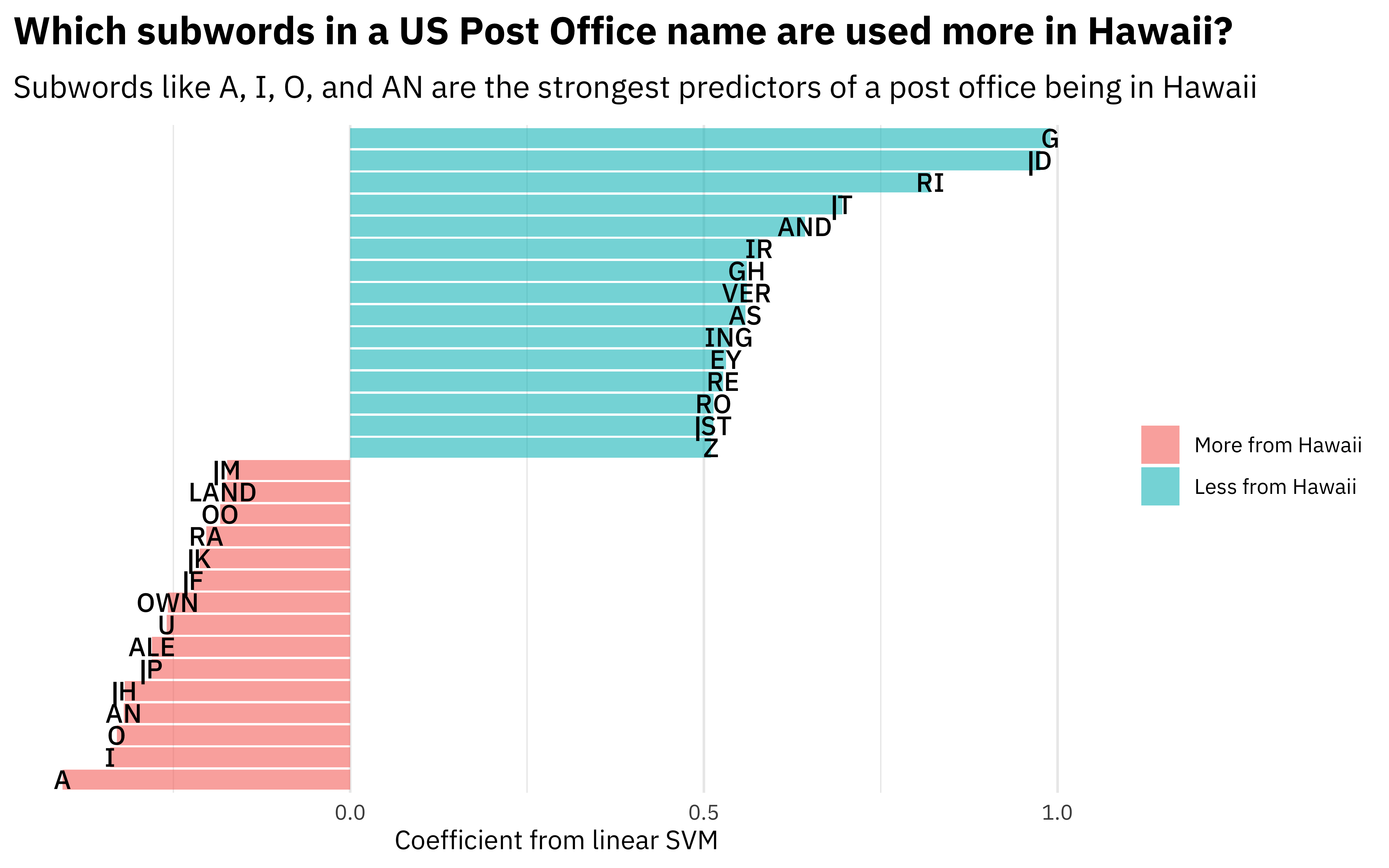
Or we can build a visualization.
liblinear_df %>%
  filter(term != "Bias") %>%
  group_by(estimate > 0) %>%
  slice_max(abs(estimate), n = 15) %>%
  ungroup() %>%
  mutate(term = str_remove(term, "tf_name_")) %>%
  ggplot(aes(estimate, fct_reorder(term, estimate), fill = estimate > 0)) +
  geom_col(alpha = 0.6) +
  geom_text(aes(label = term), family = "IBMPlexSans-Medium") +
  scale_fill_discrete(labels = c("More from Hawaii", "Less from Hawaii")) +
  scale_y_discrete(breaks = NULL) +
  theme(axis.text.y = element_blank()) +
  labs(
    x = "Coefficient from linear SVM",
    y = NULL,
    fill = NULL,
    title = "Which subwords in a US Post Office name are used more in Hawaii?",
    subtitle = "Subwords like A, I, O, and AN are the strongest predictors of a post office being in Hawaii"
  )
- Posted on:
- April 14, 2021
- Length:
- 10 minute read, 2045 words
- Categories:
- rstats tidymodels
- Tags:
- rstats tidymodels