Which #TidyTuesday Netflix titles are movies and which are TV shows?
By Julia Silge in rstats tidymodels
April 23, 2021
This is the latest in my series of
screencasts demonstrating how to use the
tidymodels packages, from just starting out to tuning more complex models with many hyperparameters. Today’s screencast walks through how to build features for modeling from text, with this week’s
#TidyTuesday dataset on Netflix titles. 📺
Here is the code I used in the video, for those who prefer reading instead of or in addition to video.
Explore data
Our modeling goal is to predict whether a title on Netflix is a TV show or a movie based on its description in this week’s #TidyTuesday dataset.
Let’s start by reading in the data.
library(tidyverse)

netflix_titles <- read_csv("https://raw.githubusercontent.com/rfordatascience/tidytuesday/master/data/2021/2021-04-20/netflix_titles.csv")
How many titles are there in this data set?
netflix_titles %>%
  count(type)
## # A tibble: 2 x 2
##   type        n
##   <chr>   <int>
## 1 Movie    5377
## 2 TV Show  2410
What do the descriptions look like? It is always a good idea to actually look at your data before modeling.
netflix_titles %>%
  slice_sample(n = 10) %>%
  pull(description)
##  [1] "When sinister Dr. Pacenstein schemes to swap bodies with Pac during a Halloween party, Spiral, Cyli and Count Pacula scramble to save their pal."
##  [2] "Monstrous frights meet hilarious reveals on this hidden-camera prank show as real people become the stars of their own full-blown horror movie."
##  [3] "After faking his death, a tech billionaire recruits a team of international operatives for a bold and bloody mission to take down a brutal dictator."
##  [4] "When a confident college professor is courted by four eligible and well-established men, she struggles to decide who she likes the best."
##  [5] "When a gay brainiac with OCD questions his identity, he enters a romantic relationship with a woman, leaving sex and physical intimacy out of it."
##  [6] "When her class rank threatens her college plans, an ambitious teen convinces a nerdy peer to run for the school board to abolish the ranking system."
##  [7] "In each episode, four celebrities join host Jon Favreau for dinner and share revealing stories about both show business and their personal lives."
##  [8] "After dating a charming cop who turns into an obsessive stalker, a small-town girl must save herself from his deadly ways."
##  [9] "A new part-time job forces Henry Hart to balance two lives, one as a typical teenager and the other as secret superhero sidekick Kid Danger."
## [10] "After getting a memory implant, working stiff Douglas Quaid discovers he might actually be a secret agent embroiled in a violent insurrection on Mars."
What are the top words in each category?
library(tidytext)

netflix_titles %>%
  unnest_tokens(word, description) %>%
  anti_join(get_stopwords()) %>%
  count(type, word, sort = TRUE) %>%
  group_by(type) %>%
  slice_max(n, n = 15) %>%
  ungroup() %>%
  mutate(word = reorder_within(word, n, type)) %>%
  ggplot(aes(n, word, fill = type)) +
  geom_col(show.legend = FALSE, alpha = 0.8) +
  scale_y_reordered() +
  facet_wrap(~type, scales = "free") +
  labs(
    x = "Word frequency", y = NULL,
    title = "Top words in Netflix descriptions by frequency",
    subtitle = "After removing stop words"
  )
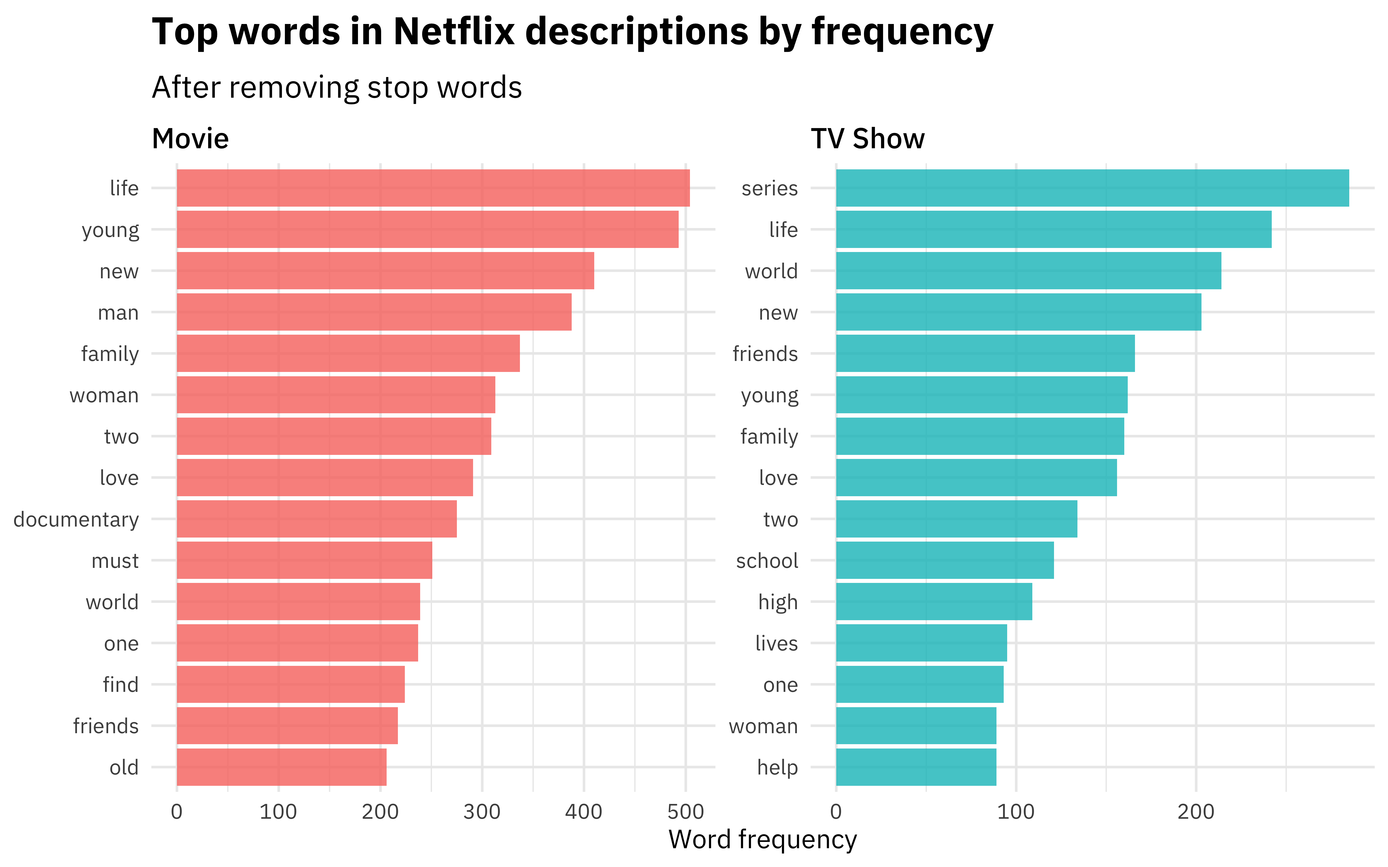
There are some differences in even the very top, most frequent words used, so hopefully we can train a model to distinguish these categories.
Build a model
We can start by loading the tidymodels metapackage, splitting our data into training and testing sets, and creating cross-validation samples. Think about this stage as spending your data budget.
library(tidymodels)

set.seed(123)
netflix_split <- netflix_titles %>%
  select(type, description) %>%
  initial_split(strata = type)

netflix_train <- training(netflix_split)
netflix_test <- testing(netflix_split)

set.seed(234)
netflix_folds <- vfold_cv(netflix_train, strata = type)
netflix_folds
## #  10-fold cross-validation using stratification
## # A tibble: 10 x 2
##    splits             id
##    <list>             <chr>
##  1 <split [5256/585]> Fold01
##  2 <split [5256/585]> Fold02
##  3 <split [5256/585]> Fold03
##  4 <split [5257/584]> Fold04
##  5 <split [5257/584]> Fold05
##  6 <split [5257/584]> Fold06
##  7 <split [5257/584]> Fold07
##  8 <split [5257/584]> Fold08
##  9 <split [5258/583]> Fold09
## 10 <split [5258/583]> Fold10
Next, let’s create our feature engineering recipe and our model, and then put them together in a modeling workflow. This feature engineering recipe is a good basic default for a text model, but you can read more about creating features from text in my book with Emil Hvitfeldt, Supervised Machine Learning for Text Analysis in R.
library(textrecipes)
library(themis)

netflix_rec <- recipe(type ~ description, data = netflix_train) %>%
  step_tokenize(description) %>%
  step_tokenfilter(description, max_tokens = 1e3) %>%
  step_tfidf(description) %>%
  step_normalize(all_numeric_predictors()) %>%
  step_smote(type)

netflix_rec
## Data Recipe
##
## Inputs:
##
##       role #variables
##    outcome          1
##  predictor          1
##
## Operations:
##
## Tokenization for description
## Text filtering for description
## Term frequency-inverse document frequency with description
## Centering and scaling for all_numeric_predictors()
## SMOTE based on type
svm_spec <- svm_linear() %>%
  set_mode("classification") %>%
  set_engine("LiblineaR")

netflix_wf <- workflow() %>%
  add_recipe(netflix_rec) %>%
  add_model(svm_spec)

netflix_wf
## ══ Workflow ════════════════════════════════════════════════════════════════════
## Preprocessor: Recipe
## Model: svm_linear()
##
## ── Preprocessor ────────────────────────────────────────────────────────────────
## 5 Recipe Steps
##
## ● step_tokenize()
## ● step_tokenfilter()
## ● step_tfidf()
## ● step_normalize()
## ● step_smote()
##
## ── Model ───────────────────────────────────────────────────────────────────────
## Linear Support Vector Machine Specification (classification)
##
## Computational engine: LiblineaR
This linear support vector machine is a newer model in parsnip, currently in the development version on GitHub. Linear SVMs are often a good starting choice for text models. When you use an SVM, remember to step_normalize()!
Now let’s fit this workflow (that combines feature engineering with the SVM model) to the resamples we created earlier. The linear SVM model does not support class probabilities, so we need to set a custom metric_set() that only includes metrics for hard class probabilities.
doParallel::registerDoParallel()
set.seed(123)
svm_rs <- fit_resamples(
  netflix_wf,
  netflix_folds,
  metrics = metric_set(accuracy, recall, precision),
  control = control_resamples(save_pred = TRUE)
)

collect_metrics(svm_rs)
## # A tibble: 3 x 6
##   .metric   .estimator  mean     n std_err .config
##   <chr>     <chr>      <dbl> <int>   <dbl> <chr>
## 1 accuracy  binary     0.680    10 0.00457 Preprocessor1_Model1
## 2 precision binary     0.791    10 0.00341 Preprocessor1_Model1
## 3 recall    binary     0.729    10 0.00592 Preprocessor1_Model1
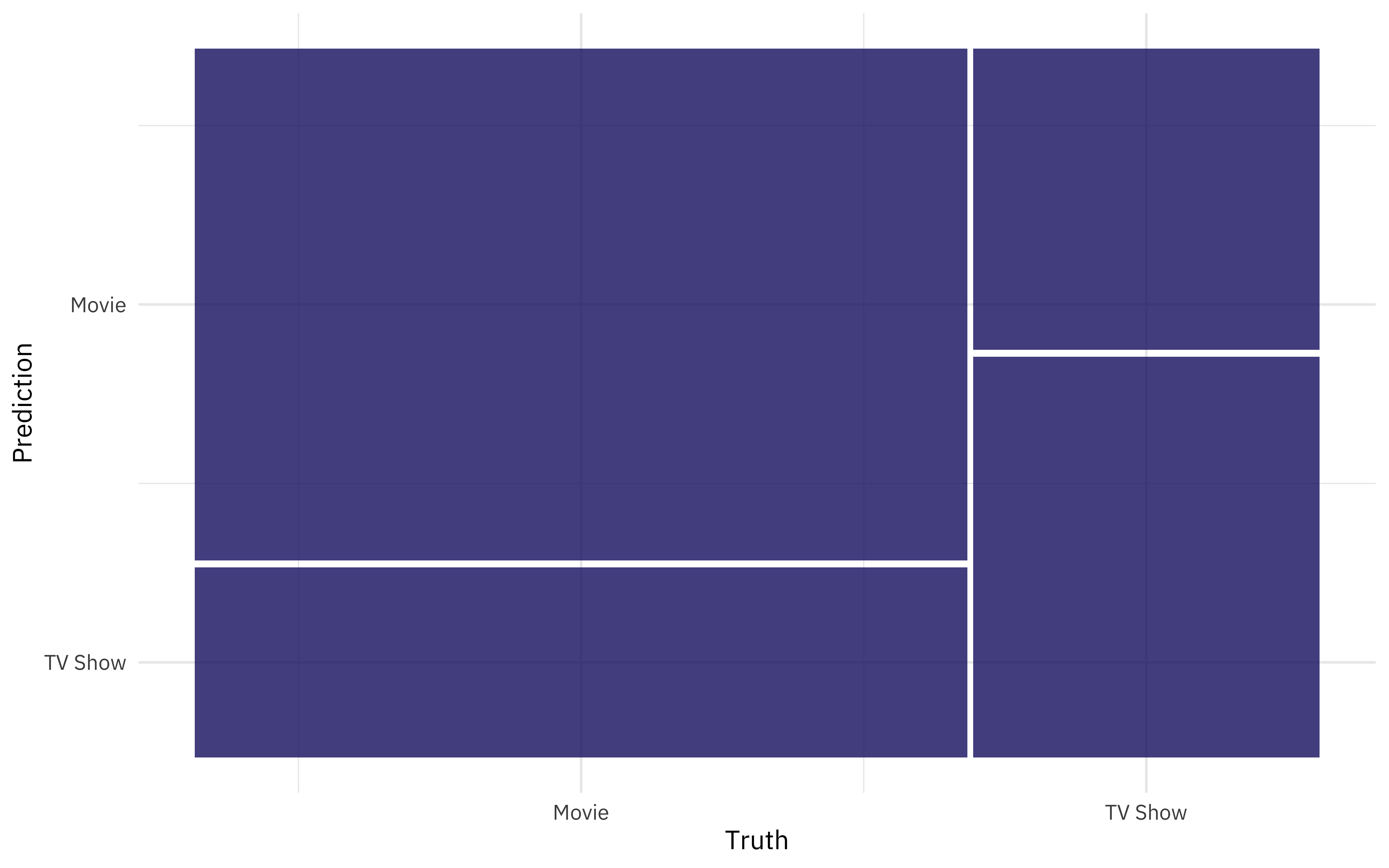
We can use
conf_mat_resampled() to compute a separate confusion matrix for each resample, and then average the cell counts.
svm_rs %>%
  conf_mat_resampled(tidy = FALSE) %>%
  autoplot()
Fit and evaluate final model
Next, let’s fit our model on last time to the whole training set at once (rather than resampled data) and evaluate on the testing set. This is the first time we have touched the testing set.
final_fitted <- last_fit(
  netflix_wf,
  netflix_split,
  metrics = metric_set(accuracy, recall, precision)
)
collect_metrics(final_fitted)
## # A tibble: 3 x 4
##   .metric   .estimator .estimate .config
##   <chr>     <chr>          <dbl> <chr>
## 1 accuracy  binary         0.685 Preprocessor1_Model1
## 2 recall    binary         0.734 Preprocessor1_Model1
## 3 precision binary         0.794 Preprocessor1_Model1
Our performance on the testing set is about the same as what we found with our resampled data, which is good.
We can explore how the model is doing for both the positive and negative classes with a confusion matrix.
collect_predictions(final_fitted) %>%
  conf_mat(type, .pred_class)
##           Truth
## Prediction Movie TV Show
##    Movie     987     256
##    TV Show   357     346
There is a fitted workflow in the .workflow column of the final_fitted tibble that can be saved and used for prediction later. Here, let’s pull out the parsnip fit and learn about model explanations.
netflix_fit <- pull_workflow_fit(final_fitted$.workflow[[1]])

tidy(netflix_fit) %>%
  arrange(estimate)
## # A tibble: 1,001 x 2
##    term                          estimate
##    <chr>                            <dbl>
##  1 Bias                           -0.362
##  2 tfidf_description_documentary  -0.200
##  3 tfidf_description_biopic       -0.176
##  4 tfidf_description_performance  -0.137
##  5 tfidf_description_how          -0.107
##  6 tfidf_description_stand        -0.104
##  7 tfidf_description_comic        -0.103
##  8 tfidf_description_mr           -0.0941
##  9 tfidf_description_film         -0.0916
## 10 tfidf_description_summer       -0.0905
## # … with 991 more rows
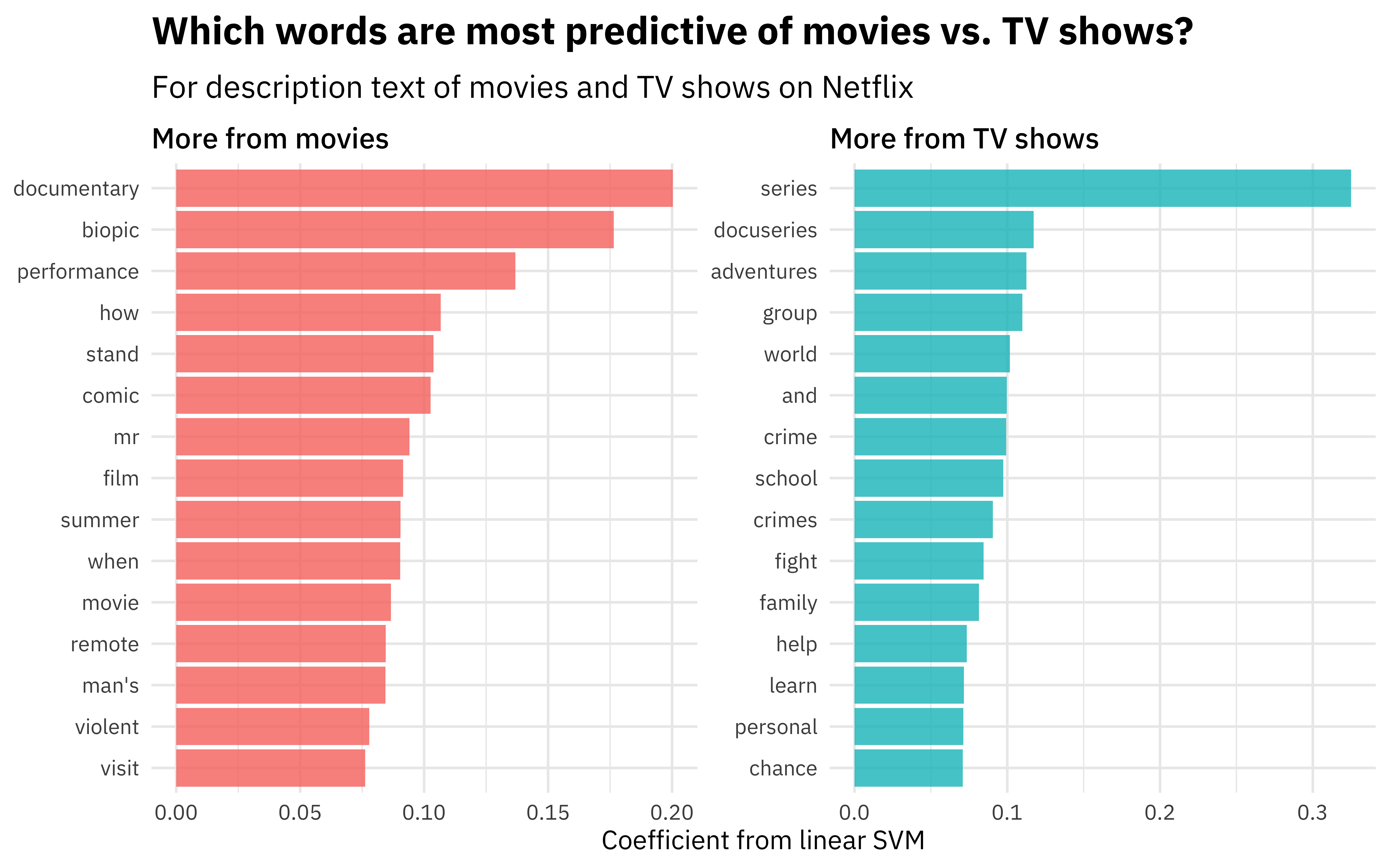
Those term items are the word features that we created during feature engineering. Let’s set up a visualization to see them better.
tidy(netflix_fit) %>%
  filter(term != "Bias") %>%
  group_by(sign = estimate > 0) %>%
  slice_max(abs(estimate), n = 15) %>%
  ungroup() %>%
  mutate(
    term = str_remove(term, "tfidf_description_"),
    sign = if_else(sign, "More from TV shows", "More from movies")
  ) %>%
  ggplot(aes(abs(estimate), fct_reorder(term, abs(estimate)), fill = sign)) +
  geom_col(alpha = 0.8, show.legend = FALSE) +
  facet_wrap(~sign, scales = "free") +
  labs(
    x = "Coefficient from linear SVM", y = NULL,
    title = "Which words are most predictive of movies vs. TV shows?",
    subtitle = "For description text of movies and TV shows on Netflix"
  )
- Posted on:
- April 23, 2021
- Length:
- 7 minute read, 1385 words
- Categories:
- rstats tidymodels
- Tags:
- rstats tidymodels