Introducing tidylo
By Julia Silge
July 8, 2019
Today I am so pleased to introduce a new package for calculating weighted log odds ratios, tidylo.
Often in data analysis, we want to measure how the usage or frequency of some feature, such as words, differs across some group or set, such as documents. One statistic often used to find these kinds of differences in text data is tf-idf. Another option is to use the log odds ratio, but the log odds ratio alone does not account for sampling variability. We haven’t counted every feature the same number of times so how do we know which differences are meaningful? 🤔
Weighty business
Instead, we can use a weighted log odds, which tidylo provides an implementation for using tidy data principles. In particular, this package uses the method outlined in Monroe, Colaresi, and Quinn (2008) to weight the log odds ratio by an uninformative Dirichlet prior.
I started developing this package with Tyler Schnoebelen after he wrote a post which I highly recommend that you go read, titled “I dare say you will never use tf-idf again”.
It starts:
Julia Silge, astrophysicist, R guru and maker of beautiful charts, a data scientist with what seem by any account to be comfortable and happy cats, united the best blessings of existence; and had lived in the world with very little to distress or vex her.
Let’s just say it gets better from there. AND it walks through the benefits of using a weighted log odds ratio for text analysis when the analytical question is focused on differences in frequency across sets, in this particular case, books.
Tyler and I have collaborated on this package implementing this approach, and it is now available on GitHub. You can install it via remotes.
library(remotes)
install_github("juliasilge/tidylo")
Tyler and I think that “tidylo” is pronounced “tidy-low”, or maybe, if you prefer, “tidy-el-oh”.
Some examples
The package contains examples in the README and vignette, but let’s walk though another, different example here. This weighted log odds approach is useful for text analysis, but not only for text analysis. In the weeks since we’ve had this package up and running, I’ve found myself reaching for it in multiple situations, both text and not, in my real-life day job. For this example, let’s look at the same data as my last post, names given to children in the US.
Which names were most common in the 1950s, 1960s, 1970s, and 1980?
library(tidyverse)
library(babynames)

top_names <- babynames %>%
    filter(year >= 1950,
           year < 1990) %>%
    mutate(decade = (year %/% 10) * 10,
           decade = paste0(decade, "s")) %>%
    group_by(decade) %>%
    count(name, wt = n, sort = TRUE) %>%
    ungroup

top_names
## # A tibble: 100,527 x 3
## decade name n
## <chr> <chr> <int>
## 1 1950s James 846042
## 2 1950s Michael 839459
## 3 1960s Michael 836934
## 4 1950s Robert 832336
## 5 1950s John 799658
## 6 1950s David 771242
## 7 1960s David 736583
## 8 1960s John 716284
## 9 1970s Michael 712722
## 10 1960s James 687905
## # … with 100,517 more rowsNow let’s use the bind_log_odds() function from the tidylo package to find the weighted log odds for each name. What are the highest log odds names for these decades?
library(tidylo)

name_log_odds <- top_names %>%
  bind_log_odds(decade, name, n)

name_log_odds %>%
  arrange(-log_odds)
## # A tibble: 100,527 x 4
## decade name n log_odds
## <chr> <chr> <int> <dbl>
## 1 1980s Ashley 357385 477.
## 2 1980s Jessica 471493 457.
## 3 1950s Linda 565481 414.
## 4 1980s Joshua 399131 412.
## 5 1980s Amanda 370873 391.
## 6 1970s Jason 465402 374.
## 7 1980s Justin 291843 363.
## 8 1950s Deborah 431302 348.
## 9 1980s Brandon 234294 331.
## 10 1970s Jennifer 583692 330.
## # … with 100,517 more rowsThese are the highest log odds names (names more likely to come from each decade, compared to the decades) when we have used weighting to account for sampling variability.
We can make some visualizations to understand our results better. For example, which names are most characteristic of each decade?
name_log_odds %>%
    group_by(decade) %>%
    top_n(10, log_odds) %>%
    ungroup %>%
    mutate(decade = as.factor(decade),
           name = fct_reorder(name, log_odds)) %>%
    ggplot(aes(name, log_odds, fill = decade)) +
    geom_col(show.legend = FALSE) +
    facet_wrap(~decade, scales = "free_y") +
    coord_flip() +
    scale_y_continuous(expand = c(0,0)) +
    labs(y = "Log odds ratio, weighted by uninformative Dirichlet prior",
         x = NULL,
         title = "What were the most specific baby names to each decade?",
         subtitle = "Via US Social Security Administration")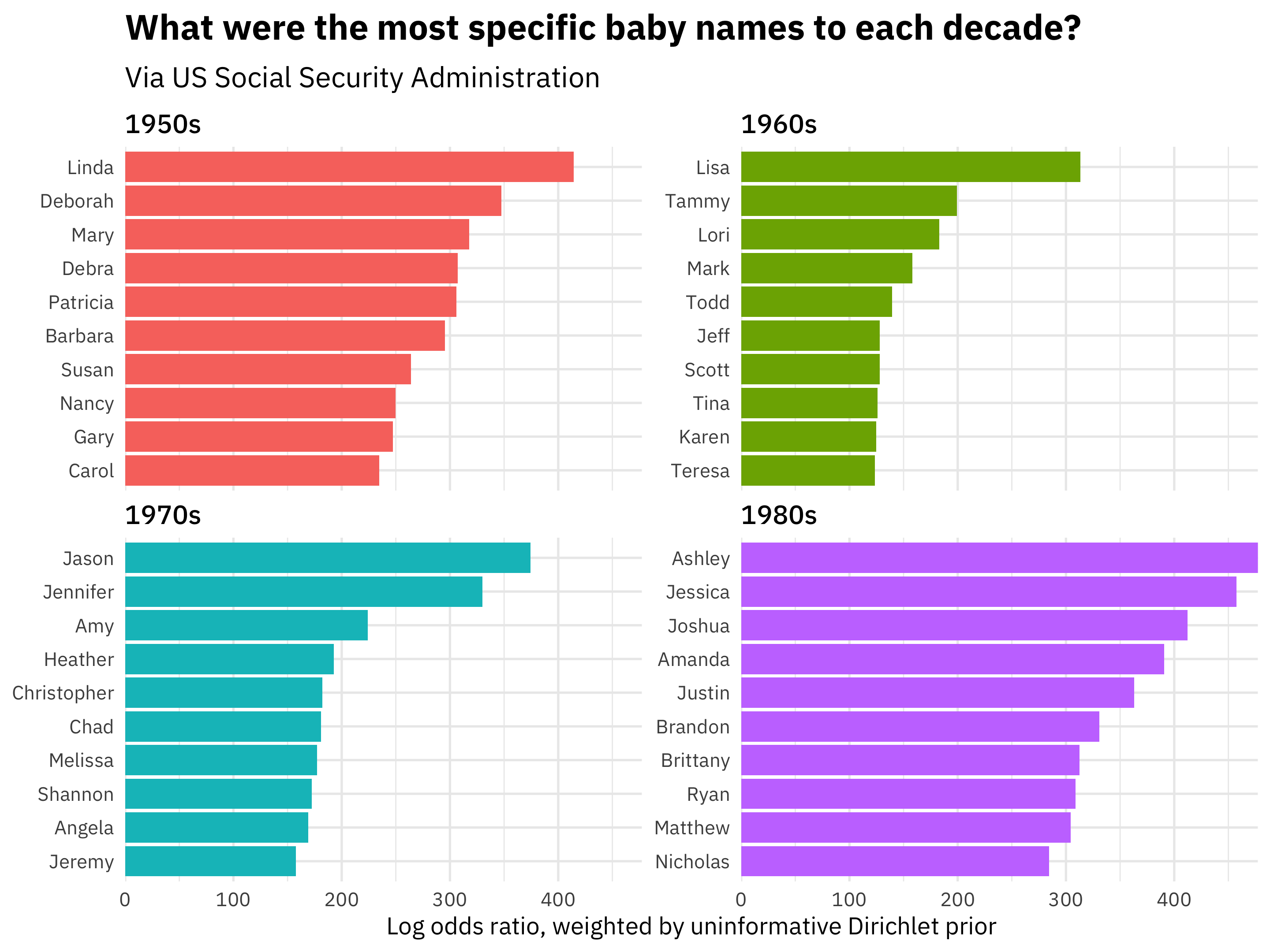
Wow, just reading those lists of names, I can picture how old those people are. I’m a child of the 1970s myself, and my childhood classrooms were in fact filled with Jasons, Jennifers, and Amys. Also notice that the weighted log odds ratios are higher in the 1980s than the other decades; the 1980s names are more different than the other decades’ names.
Perhaps we want to understand one decade more deeply. For example, what are the most 1980s names, along with how common they were?
library(ggrepel)

name_log_odds %>%
    filter(decade == "1980s") %>%
    top_n(50, n) %>%
    ggplot(aes(n, log_odds, label = name)) +
    geom_hline(yintercept = 0, lty = 2,
               color = "gray50", alpha = 0.5, size = 1.2) +
    geom_text_repel(family = "IBMPlexSans") +
    geom_point() +
    scale_x_log10() +
    labs(x = "Number of babies per decade",
         y = "Log odds ratio, weighted by uninformative Dirichlet prior",
         title = "What are the baby names most specific to the 1980s?",
         subtitle = "Via US Social Security Administration")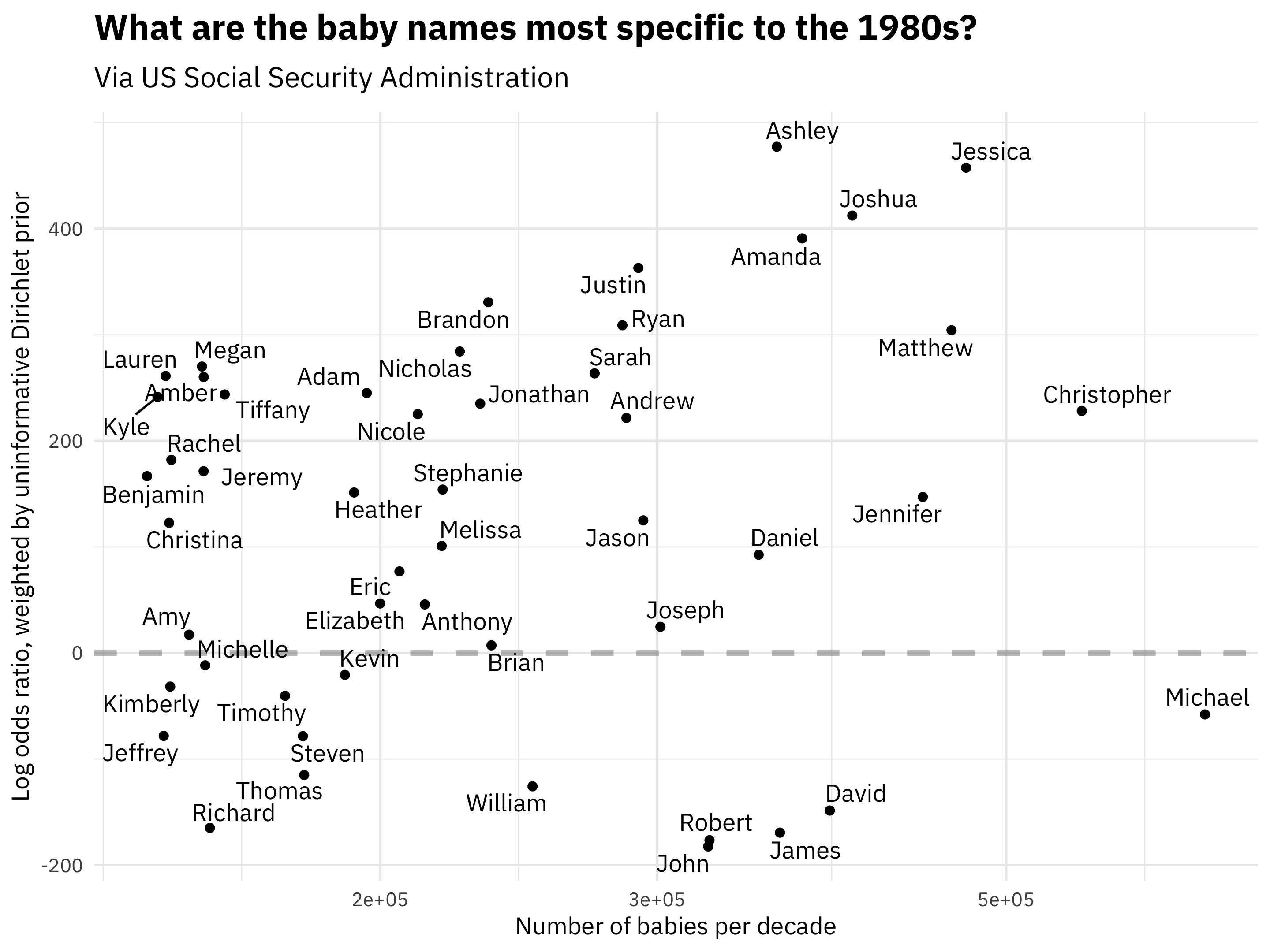
Michael is the most popular name in the 1980s, but it is not particularly likely to be used in the 1980s compared to the other decades (it was common in other decades too). We can see in this visualization the distribution of frequency and log odds ratio.
Conclusion
Give this package a try and let us know if you run into problems! We do plan to release this on CRAN later in the year, after it is stable and tested a bit in the real world.