Partial dependence plots with tidymodels and DALEX for #TidyTuesday Mario Kart world records

This is the latest in my series of screencasts demonstrating how to use the tidymodels packages, from just starting out to tuning more complex models with many hyperparameters. Today’s screencast walks through how to train and evalute a random forest model, with this week’s #TidyTuesday dataset on Mario Kart world records. 🍄

Here is the code I used in the video, for those who prefer reading instead of or in addition to video.

Explore data

Our modeling goal is to predict whether a Mario Kart world record was achieved using a shortcut or not.

library(tidyverse)

records <- read_csv("https://raw.githubusercontent.com/rfordatascience/tidytuesday/master/data/2021/2021-05-25/records.csv")

How are the world records distributed over time, for the various tracks?

records %>%
  ggplot(aes(date, time, color = track)) +
  geom_point(alpha = 0.5, show.legend = FALSE) +
  facet_grid(rows = vars(type), cols = vars(shortcut), scales = "free_y")

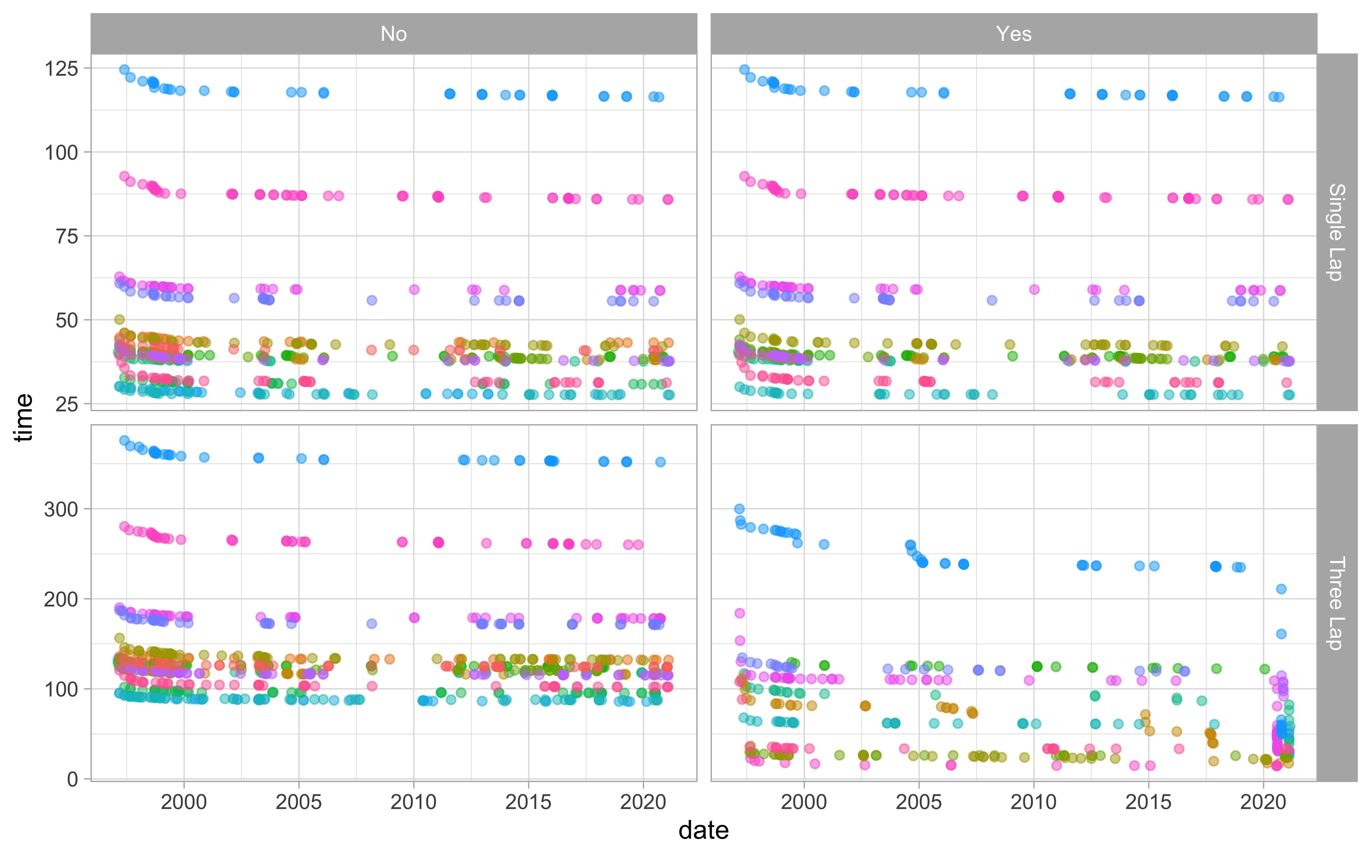
The record times decreased at first but then have been more stable. The record times are different for the different tracks, and for three lap vs. one lap times.

Build a model

Let’s start our modeling by setting up our “data budget.”

library(tidymodels)

set.seed(123)
mario_split <- records %>%
  select(shortcut, track, type, date, time) %>%
  mutate_if(is.character, factor) %>%
  initial_split(strata = shortcut)

mario_train <- training(mario_split)
mario_test <- testing(mario_split)

set.seed(234)
mario_folds <- bootstraps(mario_train, strata = shortcut)
mario_folds

## # Bootstrap sampling using stratification 
## # A tibble: 25 x 2
##    splits             id         
##    <list>             <chr>      
##  1 <split [1750/627]> Bootstrap01
##  2 <split [1750/639]> Bootstrap02
##  3 <split [1750/652]> Bootstrap03
##  4 <split [1750/644]> Bootstrap04
##  5 <split [1750/648]> Bootstrap05
##  6 <split [1750/670]> Bootstrap06
##  7 <split [1750/648]> Bootstrap07
##  8 <split [1750/660]> Bootstrap08
##  9 <split [1750/645]> Bootstrap09
## 10 <split [1750/629]> Bootstrap10
## # … with 15 more rows

For this analysis, I am tuning a decision tree model. Tree-based models are very low-maintenance when it comes to data preprocessing, but single decision trees can be pretty easy to overfit.

tree_spec <- decision_tree(
  cost_complexity = tune(),
  tree_depth = tune()
) %>%
  set_engine("rpart") %>%
  set_mode("classification")

tree_grid <- grid_regular(cost_complexity(), tree_depth(), levels = 7)

mario_wf <- workflow() %>%
  add_model(tree_spec) %>%
  add_formula(shortcut ~ .)

mario_wf

## ══ Workflow ════════════════════════════════════════════════════════════════════
## Preprocessor: Formula
## Model: decision_tree()
## 
## ── Preprocessor ────────────────────────────────────────────────────────────────
## shortcut ~ .
## 
## ── Model ───────────────────────────────────────────────────────────────────────
## Decision Tree Model Specification (classification)
## 
## Main Arguments:
##   cost_complexity = tune()
##   tree_depth = tune()
## 
## Computational engine: rpart

Let’s tune the tree parameters to find the best decision tree for this Mario Kart data set.

doParallel::registerDoParallel()

tree_res <- tune_grid(
  mario_wf,
  resamples = mario_folds,
  grid = tree_grid,
  control = control_grid(save_pred = TRUE)
)

tree_res

## # Tuning results
## # Bootstrap sampling using stratification 
## # A tibble: 25 x 5
##    splits           id         .metrics        .notes        .predictions       
##    <list>           <chr>      <list>          <list>        <list>             
##  1 <split [1750/62… Bootstrap… <tibble [98 × … <tibble [0 ×… <tibble [30,723 × …
##  2 <split [1750/63… Bootstrap… <tibble [98 × … <tibble [0 ×… <tibble [31,311 × …
##  3 <split [1750/65… Bootstrap… <tibble [98 × … <tibble [0 ×… <tibble [31,948 × …
##  4 <split [1750/64… Bootstrap… <tibble [98 × … <tibble [0 ×… <tibble [31,556 × …
##  5 <split [1750/64… Bootstrap… <tibble [98 × … <tibble [0 ×… <tibble [31,752 × …
##  6 <split [1750/67… Bootstrap… <tibble [98 × … <tibble [0 ×… <tibble [32,830 × …
##  7 <split [1750/64… Bootstrap… <tibble [98 × … <tibble [0 ×… <tibble [31,752 × …
##  8 <split [1750/66… Bootstrap… <tibble [98 × … <tibble [0 ×… <tibble [32,340 × …
##  9 <split [1750/64… Bootstrap… <tibble [98 × … <tibble [0 ×… <tibble [31,605 × …
## 10 <split [1750/62… Bootstrap… <tibble [98 × … <tibble [0 ×… <tibble [30,821 × …
## # … with 15 more rows

All done! We tried all the possible combinations of tree parameters for each resample.

Choose and evaluate final model

Now we can explore our tuning results.

collect_metrics(tree_res)

## # A tibble: 98 x 8
##    cost_complexity tree_depth .metric  .estimator  mean     n std_err .config   
##              <dbl>      <int> <chr>    <chr>      <dbl> <int>   <dbl> <chr>     
##  1   0.0000000001           1 accuracy binary     0.637    25 0.00371 Preproces…
##  2   0.0000000001           1 roc_auc  binary     0.637    25 0.0109  Preproces…
##  3   0.00000000316          1 accuracy binary     0.637    25 0.00371 Preproces…
##  4   0.00000000316          1 roc_auc  binary     0.637    25 0.0109  Preproces…
##  5   0.0000001              1 accuracy binary     0.637    25 0.00371 Preproces…
##  6   0.0000001              1 roc_auc  binary     0.637    25 0.0109  Preproces…
##  7   0.00000316             1 accuracy binary     0.637    25 0.00371 Preproces…
##  8   0.00000316             1 roc_auc  binary     0.637    25 0.0109  Preproces…
##  9   0.0001                 1 accuracy binary     0.637    25 0.00371 Preproces…
## 10   0.0001                 1 roc_auc  binary     0.637    25 0.0109  Preproces…
## # … with 88 more rows

show_best(tree_res, metric = "accuracy")

## # A tibble: 5 x 8
##   cost_complexity tree_depth .metric  .estimator  mean     n std_err .config    
##             <dbl>      <int> <chr>    <chr>      <dbl> <int>   <dbl> <chr>      
## 1   0.00316                8 accuracy binary     0.738    25 0.00248 Preprocess…
## 2   0.0000000001           8 accuracy binary     0.736    25 0.00249 Preprocess…
## 3   0.00000000316          8 accuracy binary     0.736    25 0.00249 Preprocess…
## 4   0.0000001              8 accuracy binary     0.736    25 0.00249 Preprocess…
## 5   0.00000316             8 accuracy binary     0.736    25 0.00249 Preprocess…

autoplot(tree_res)

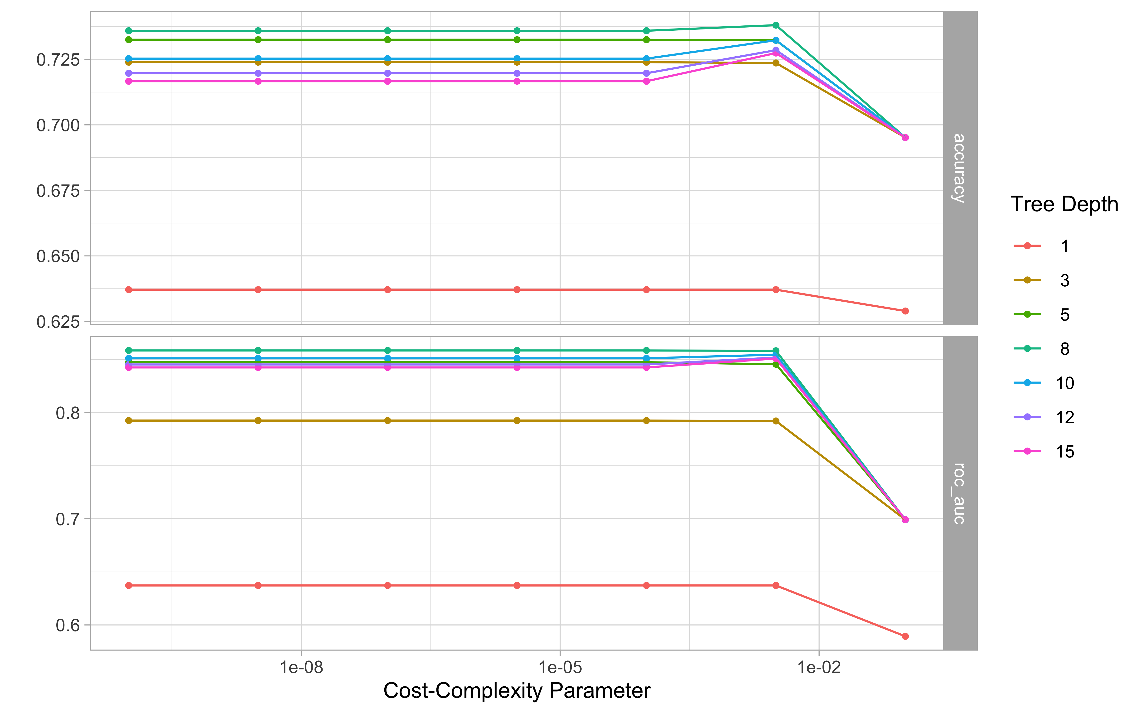
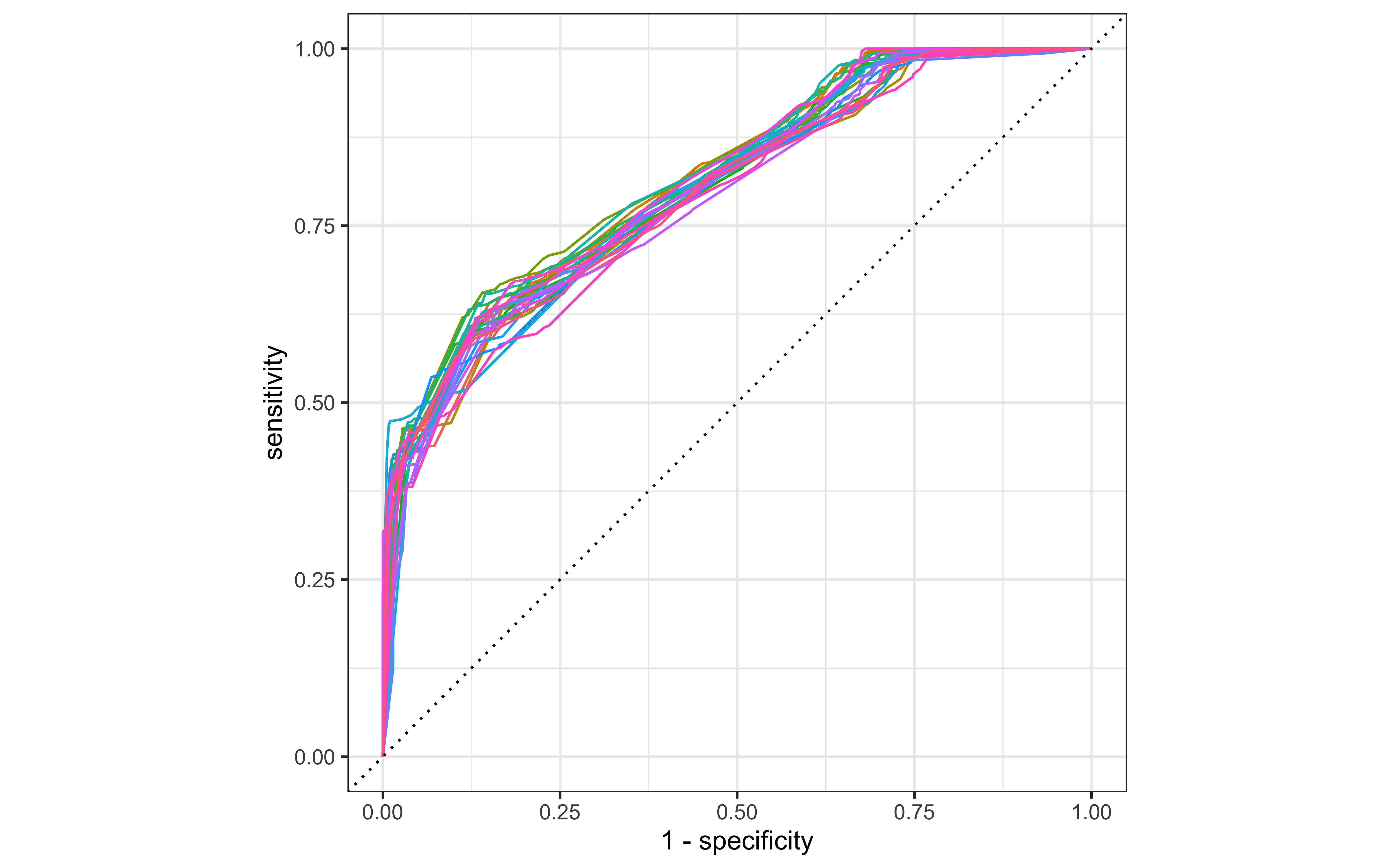
Looks like a tree depth of 8 is best. How do the ROC curves look for the resampled training set?

collect_predictions(tree_res) %>%
  group_by(id) %>%
  roc_curve(shortcut, .pred_No) %>%
  autoplot() +
  theme(legend.position = "none")

Let’s choose the tree parameters we want to use, finalize our (tuneable) workflow with this choice, and then fit one last time to the training data and evaluate on the testing data. This is the first time we have used the test set.

choose_tree <- select_best(tree_res, metric = "accuracy")

final_res <- mario_wf %>%
  finalize_workflow(choose_tree) %>%
  last_fit(mario_split)

collect_metrics(final_res)

## # A tibble: 2 x 4
##   .metric  .estimator .estimate .config             
##   <chr>    <chr>          <dbl> <chr>               
## 1 accuracy binary         0.721 Preprocessor1_Model1
## 2 roc_auc  binary         0.847 Preprocessor1_Model1

One of the objects contained in final_res is a fitted workflow that we can save for future use or deployment (perhaps via readr::write_rds()) and use for prediction on new data.

final_fitted <- final_res$.workflow[[1]]
predict(final_fitted, mario_test[10:12, ])

## # A tibble: 3 x 1
##   .pred_class
##   <fct>      
## 1 No         
## 2 No         
## 3 Yes

We can use this fitted workflow to explore model explainability as well. Decision trees are pretty explainable already, but we might, for example, want to see a partial dependence plot for the shortcut probability and time. I like using the DALEX package for tasks like this, because it is very fully featured and has good support for tidymodels. To use DALEX with tidymodels, first you create an explainer and then you use that explainer for the task you want, like computing a PDP or Shapley explanations.

Let’s start by creating our “explainer.”

library(DALEXtra)

mario_explainer <- explain_tidymodels(
  final_fitted,
  data = dplyr::select(mario_train, -shortcut),
  y = as.integer(mario_train$shortcut),
  verbose = FALSE
)

Then let’s compute a partial dependence profile for time, grouped by type, which is three laps vs. one lap.

pdp_time <- model_profile(
  mario_explainer,
  variables = "time",
  N = NULL,
  groups = "type"
)

You can use the default plotting from DALEX by calling plot(pdp_time), but if you like to customize your plots, you can access the underlying data via pdp_time$agr_profiles and pdp_time$cp_profiles.

as_tibble(pdp_time$agr_profiles) %>%
  mutate(`_label_` = str_remove(`_label_`, "workflow_")) %>%
  ggplot(aes(`_x_`, `_yhat_`, color = `_label_`)) +
  geom_line(size = 1.2, alpha = 0.8) +
  labs(
    x = "Time to complete track",
    y = "Predicted probability of shortcut",
    color = NULL,
    title = "Partial dependence plot for Mario Kart world records",
    subtitle = "Predictions from a decision tree model"
  )

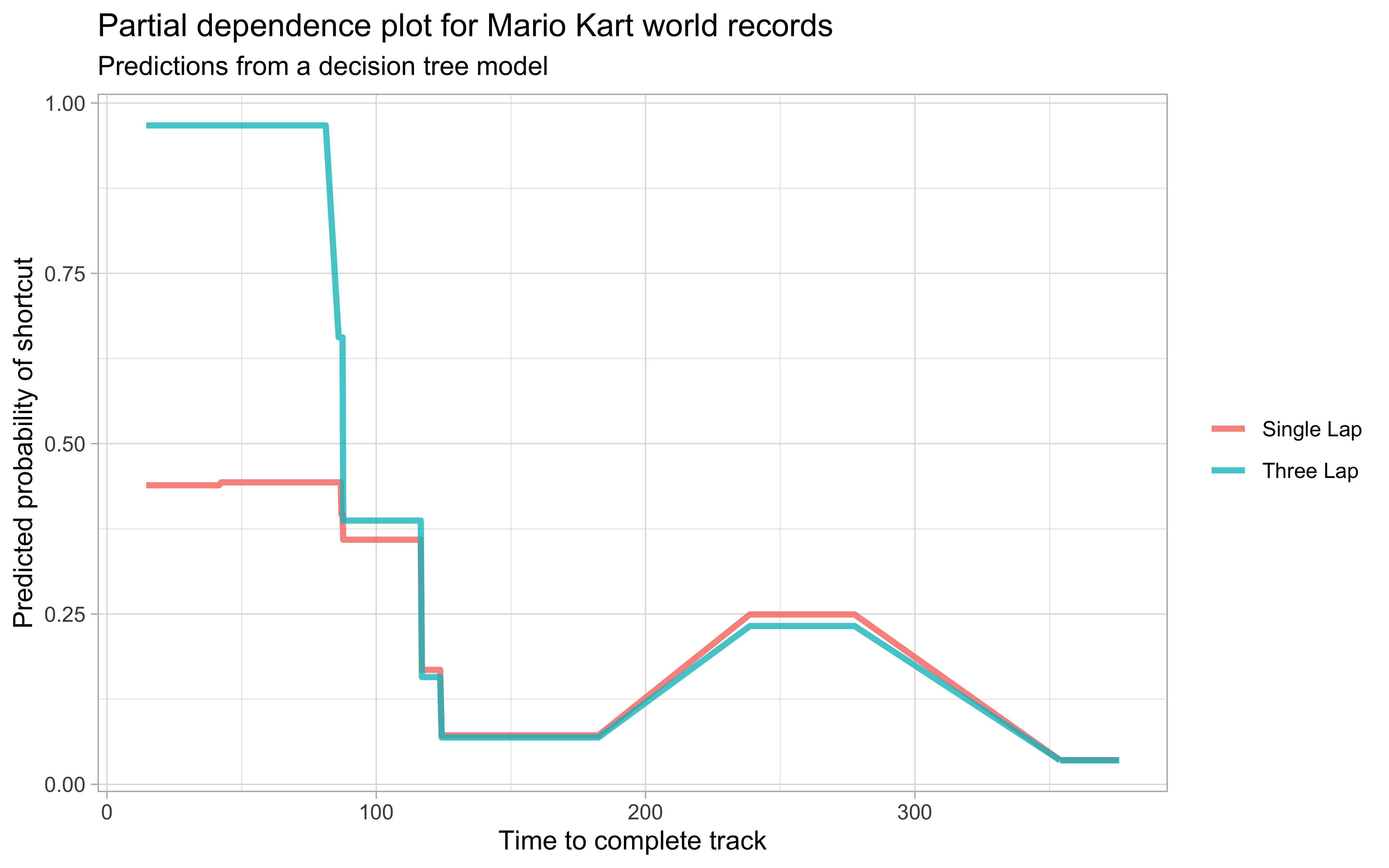
The shapes that we see here reflect how the decision tree model makes decisions along the time variable.