Create a custom metric with tidymodels and NYC Airbnb prices
By Julia Silge in rstats tidymodels
June 30, 2021
This is the latest in my series of screencasts demonstrating how to use the tidymodels packages, from just getting started to tuning more complex models. This week’s episode of SLICED, a competitive data science prediction challenge, introduced a challenge for predicting the prices of Airbnb listings in NYC. In today’s screencast, I walk through how to build such a model combining tabular data with unstructured text data from the listing names, and how to create a custom metric in tidymodels. 🌆
Here is the code I used in the video, for those who prefer reading instead of or in addition to video.
Explore data
Our modeling goal is to predict
Airbnb prices in New York City given other information about the listings. This challenge was being evaluated on
RMSLE. The main data set provided is in a CSV file called training.csv.
library(tidyverse)
train_raw <- read_csv("train.csv")
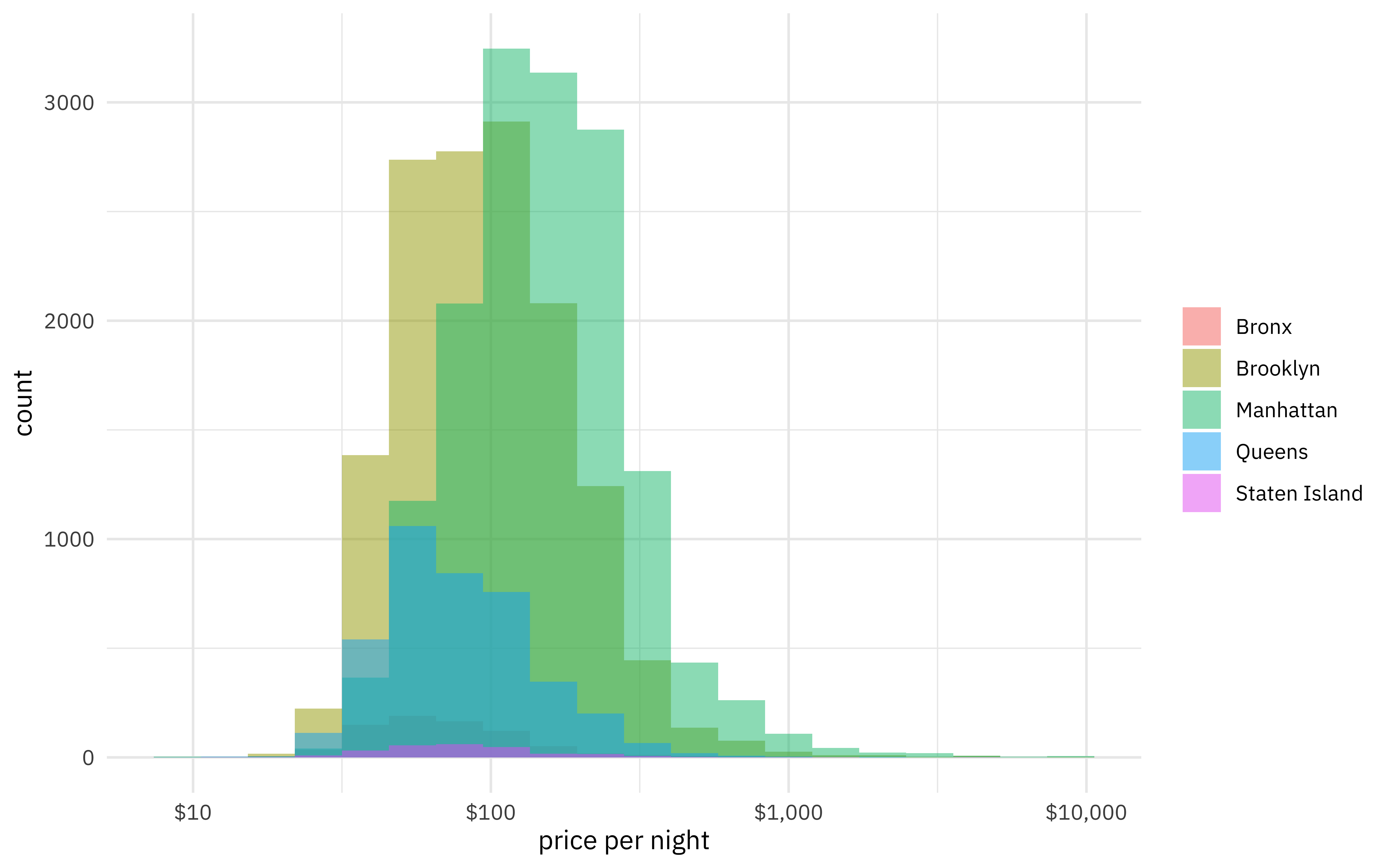
The price variable is skewed a lot, as prices often are!
train_raw %>%
  ggplot(aes(price, fill = neighbourhood_group)) +
  geom_histogram(position = "identity", alpha = 0.5, bins = 20) +
  scale_x_log10(labels = scales::dollar_format()) +
  labs(fill = NULL, x = "price per night")
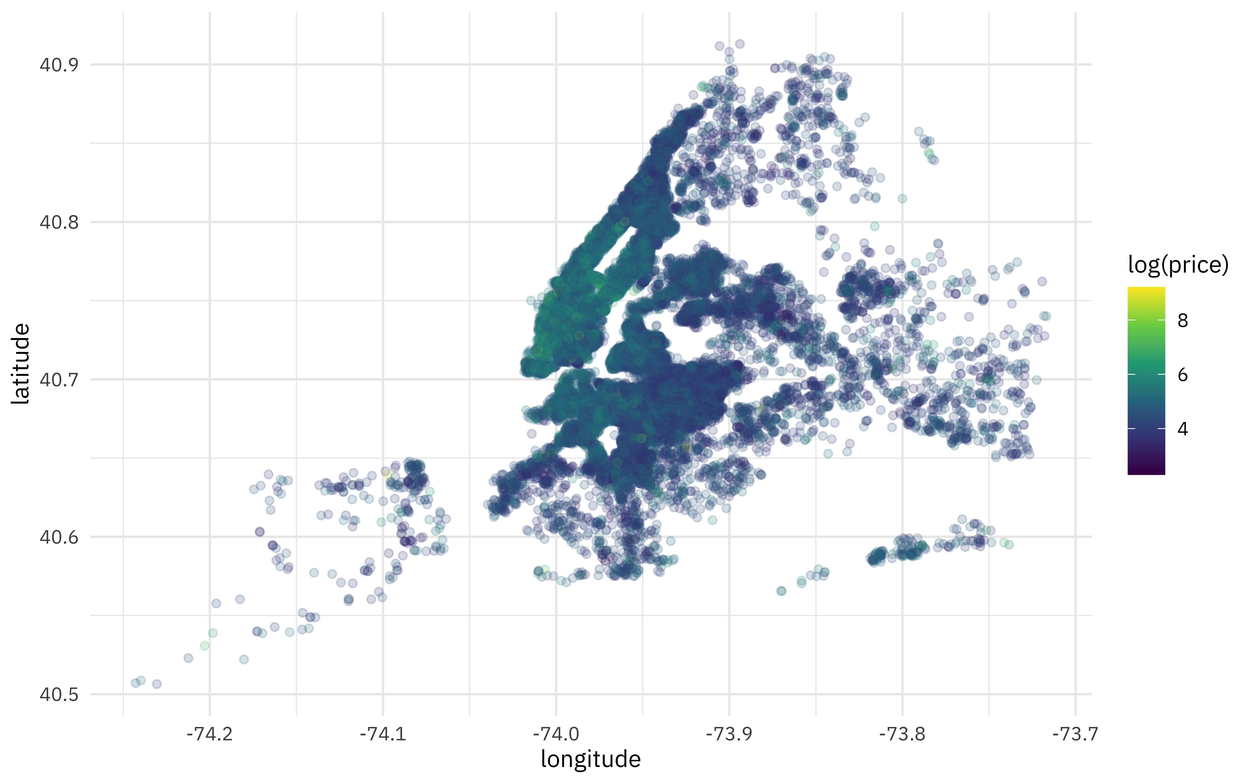
We can make a map showing each individual listing.
train_raw %>%
  ggplot(aes(longitude, latitude, color = log(price))) +
  geom_point(alpha = 0.2) +
  scale_color_viridis_c()
Or a map with hex bins showing the mean price in each area.
train_raw %>%
  ggplot(aes(longitude, latitude, z = log(price))) +
  stat_summary_hex(alpha = 0.8, bins = 70) +
  scale_fill_viridis_c() +
  labs(fill = "Mean price (log)")
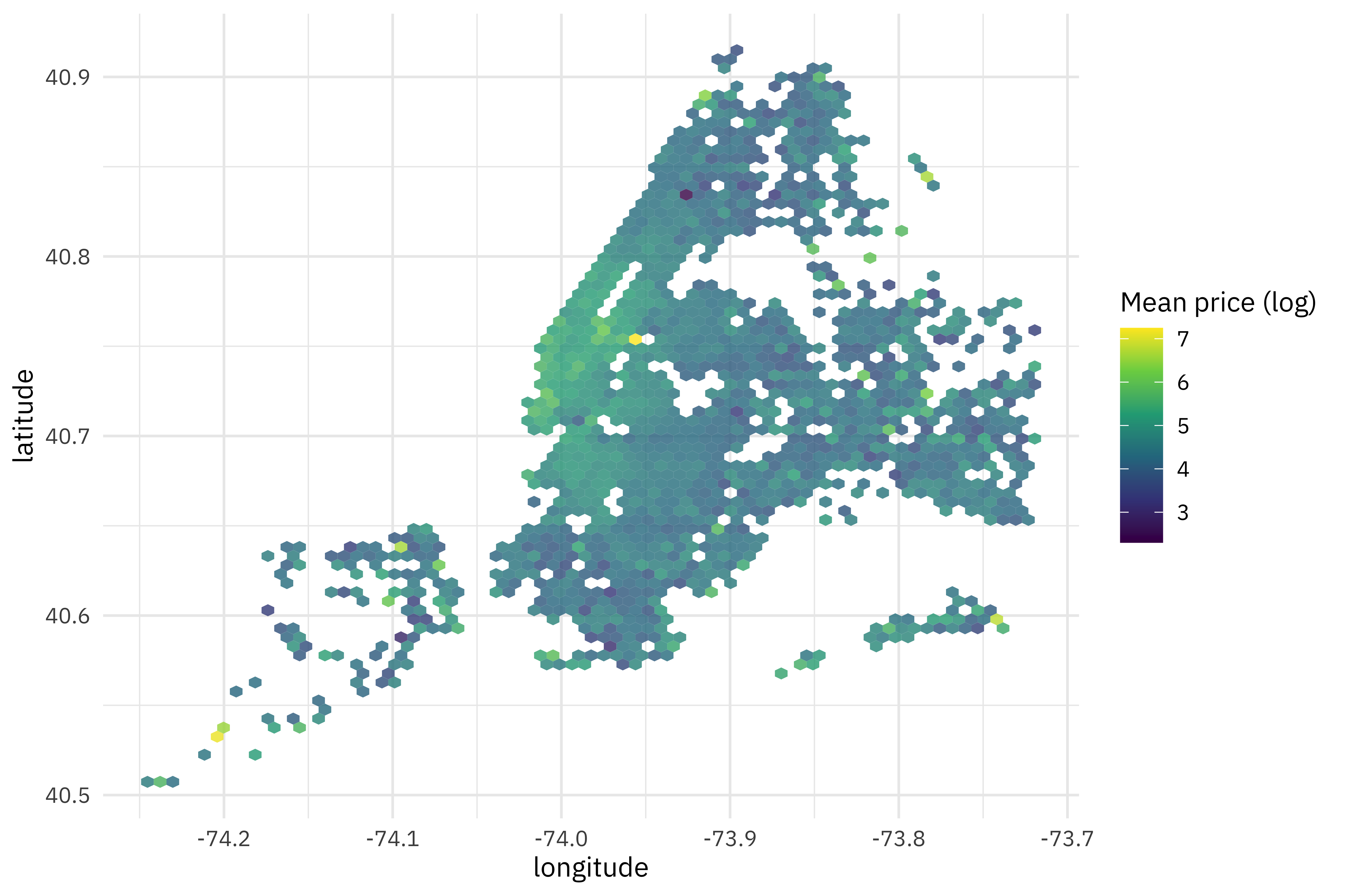
Price is definitely tied to geography!
Build a model
Let’s start by setting up our “data budget,” splitting into training and testing sets and creating resampling folds. I am going to use the testing set here to demonstrate how to use the custom metric.
library(tidymodels)

set.seed(123)
nyc_split <- train_raw %>%
  mutate(price = log(price + 1)) %>%
  initial_split(strata = price)
nyc_train <- training(nyc_split)
nyc_test <- testing(nyc_split)

set.seed(234)
nyc_folds <- vfold_cv(nyc_train, v = 5, strata = price)
nyc_folds
## #  5-fold cross-validation using stratification
## # A tibble: 5 x 2
##   splits               id
##   <list>               <chr>
## 1 <split [20533/5135]> Fold1
## 2 <split [20533/5135]> Fold2
## 3 <split [20534/5134]> Fold3
## 4 <split [20535/5133]> Fold4
## 5 <split [20537/5131]> Fold5
For feature engineering, let’s handle the many levels in neighborhood, and create features for machine learning from the text in the name variable. Read more about creating ML features from natural language
in my book with my coauthor Emil Hvitfeldt. For this demonstration, let’s start out with only the top 30 tokens and see how well we do.
library(textrecipes)

nyc_rec <-
  recipe(price ~ latitude + longitude + neighbourhood + room_type +
    minimum_nights + number_of_reviews + availability_365 + name,
  data = nyc_train
  ) %>%
  step_novel(neighbourhood) %>%
  step_other(neighbourhood, threshold = 0.01) %>%
  step_tokenize(name) %>%
  step_stopwords(name) %>%
  step_tokenfilter(name, max_tokens = 30) %>%
  step_tf(name)

nyc_rec
## Data Recipe
##
## Inputs:
##
##       role #variables
##    outcome          1
##  predictor          8
##
## Operations:
##
## Novel factor level assignment for neighbourhood
## Collapsing factor levels for neighbourhood
## Tokenization for name
## Stop word removal for name
## Text filtering for name
## Term frequency with name
For this post, let’s use a bagged tree model. It’s similar to the kinds of models that perform well in SLICED-like situations but it is easy to set up and fast to fit.
library(baguette)

bag_spec <-
  bag_tree(min_n = 10) %>%
  set_engine("rpart", times = 25) %>%
  set_mode("regression")

bag_wf <-
  workflow() %>%
  add_recipe(nyc_rec) %>%
  add_model(bag_spec)

set.seed(123)
bag_fit <- fit(bag_wf, data = nyc_train)
bag_fit
## ══ Workflow [trained] ══════════════════════════════════════════════════════════
## Preprocessor: Recipe
## Model: bag_tree()
##
## ── Preprocessor ────────────────────────────────────────────────────────────────
## 6 Recipe Steps
##
## • step_novel()
## • step_other()
## • step_tokenize()
## • step_stopwords()
## • step_tokenfilter()
## • step_tf()
##
## ── Model ───────────────────────────────────────────────────────────────────────
## Bagged CART (regression with 25 members)
##
## Variable importance scores include:
##
## # A tibble: 37 x 4
##    term              value std.error  used
##    <chr>             <dbl>     <dbl> <int>
##  1 room_type         4800.     15.5     25
##  2 longitude         3084.     13.0     25
##  3 neighbourhood     2619.     13.0     25
##  4 tf_name_room      2044.      9.17    25
##  5 latitude          1822.     14.8     25
##  6 minimum_nights    1642.      9.53    25
##  7 availability_365  1114.     10.6     25
##  8 tf_name_private    996.      7.74    25
##  9 number_of_reviews  914.      9.33    25
## 10 tf_name_studio     189.      2.99    25
## # … with 27 more rows
It’s great to automatically get out some variable importance! We see that room_type and the geographical information are very important for this model.
Evaluate a model with a custom metric
Now let’s evaluate how this model performs using resampling, first just with the default metrics for regression models.
doParallel::registerDoParallel()

set.seed(123)
bag_rs <- fit_resamples(bag_wf, nyc_folds)
collect_metrics(bag_rs)
## # A tibble: 2 x 6
##   .metric .estimator  mean     n std_err .config
##   <chr>   <chr>      <dbl> <int>   <dbl> <chr>
## 1 rmse    standard   0.437     5 0.00237 Preprocessor1_Model1
## 2 rsq     standard   0.603     5 0.00260 Preprocessor1_Model1
This might look like the values on the SLICED leaderboard, but it is RMSE on the log of price, not RMSLE on price. If I were on SLICED, I would honestly probably call this good enough TBH and not mess around with a custom metric during the competition, but it is not too difficult to extend yardstick to create a custom metric.
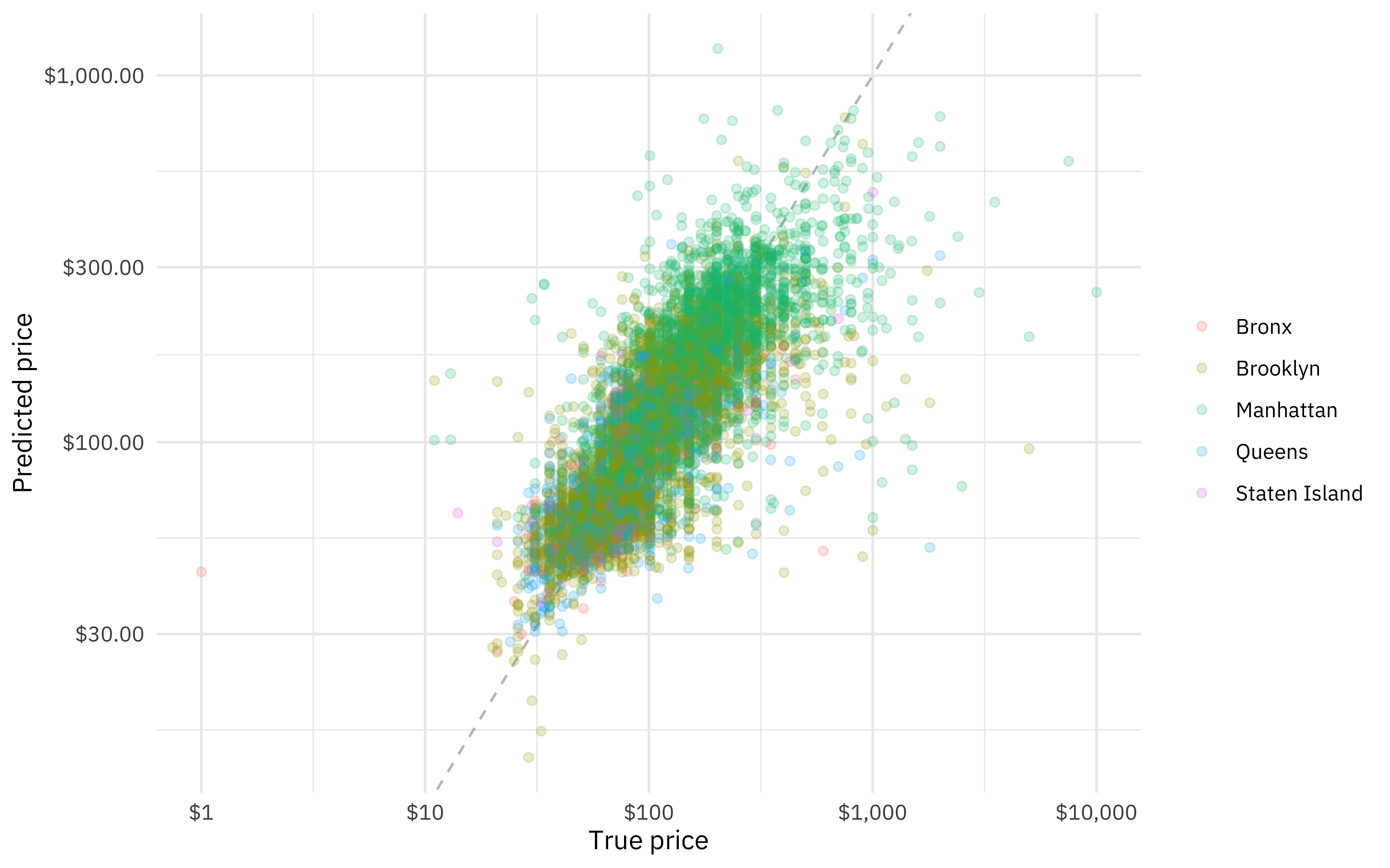
Let’s start by making some predictions on the heldout test set I created, to evaluate.
test_rs <- augment(bag_fit, nyc_test)

test_rs %>%
  ggplot(aes(exp(price), exp(.pred), color = neighbourhood_group)) +
  geom_abline(slope = 1, lty = 2, color = "gray50", alpha = 0.5) +
  geom_point(alpha = 0.2) +
  scale_x_log10(labels = scales::dollar_format()) +
  scale_y_log10(labels = scales::dollar_format()) +
  labs(color = NULL, x = "True price", y = "Predicted price")
We have an article about how to create a custom metric on tidymodels.org but the general idea is to first create a function that computes the metric for a vector and then make a method for a dataframe. Most of what’s needed for RMSLE can be taken from the functions for RMSE.
library(rlang)

rmsle_vec <- function(truth, estimate, na_rm = TRUE, ...) {
  rmsle_impl <- function(truth, estimate) {
    sqrt(mean((log(truth + 1) - log(estimate + 1))^2))
  }

  metric_vec_template(
    metric_impl = rmsle_impl,
    truth = truth,
    estimate = estimate,
    na_rm = na_rm,
    cls = "numeric",
    ...
  )
}

rmsle <- function(data, ...) {
  UseMethod("rmsle")
}
rmsle <- new_numeric_metric(rmsle, direction = "minimize")

rmsle.data.frame <- function(data, truth, estimate, na_rm = TRUE, ...) {
  metric_summarizer(
    metric_nm = "rmsle",
    metric_fn = rmsle_vec,
    data = data,
    truth = !!enquo(truth),
    estimate = !!enquo(estimate),
    na_rm = na_rm,
    ...
  )
}
Now we can apply this to our test data. In this context, we would want to use rmse() with the results on the log scale and rmsle() on the results back on the dollar scale.
test_rs %>%
  rmse(price, .pred)
## # A tibble: 1 x 3
##   .metric .estimator .estimate
##   <chr>   <chr>          <dbl>
## 1 rmse    standard       0.435
test_rs %>%
  mutate(across(c(price, .pred), exp)) %>%
  rmsle(price, .pred)
## # A tibble: 1 x 3
##   .metric .estimator .estimate
##   <chr>   <chr>          <dbl>
## 1 rmsle   standard       0.431
Not bad!
- Posted on:
- June 30, 2021
- Length:
- 6 minute read, 1164 words
- Categories:
- rstats tidymodels
- Tags:
- rstats tidymodels