Poisson regression for #TidyTuesday counts of R package vignettes

This is the latest in my series of screencasts demonstrating how to use the tidymodels packages. Our team recently released new versions of parsnip and the parsnip-adjacent packages for specialized models to CRAN, and this screencast shows how to use some of these models with the #TidyTuesday dataset on R package vignettes. 📄

Here is the code I used in the video, for those who prefer reading instead of or in addition to video.

Explore data

Our modeling goal is to understand how the number of releases and number of vignettes are related for R packages.

library(tidyverse)
cran <- read_csv("https://raw.githubusercontent.com/rfordatascience/tidytuesday/master/data/2022/2022-03-15/cran.csv")

What does this data look like, for a few packages that I maintain?

cran %>% filter(package == "tidytext")

## # A tibble: 8 × 5
##   package  version date                      rnw   rmd
##   <chr>    <chr>   <chr>                   <dbl> <dbl>
## 1 tidytext 0.2.1   2019-06-13 23:16:09 UTC     0     4
## 2 tidytext 0.2.2   2019-07-27 18:53:23 UTC     0     4
## 3 tidytext 0.2.3   2020-03-04 03:57:15 UTC     0     4
## 4 tidytext 0.2.4   2020-04-17 15:48:56 UTC     0     4
## 5 tidytext 0.2.5   2020-07-11 19:37:44 UTC     0     4
## 6 tidytext 0.2.6   2020-09-20 17:33:49 UTC     0     3
## 7 tidytext 0.3.0   2021-01-05 17:36:28 UTC     0     3
## 8 tidytext 0.3.1   2021-04-10 17:45:23 UTC     0     3

cran %>% filter(package == "rsample")

## # A tibble: 9 × 5
##   package version date                      rnw   rmd
##   <chr>   <chr>   <chr>                   <dbl> <dbl>
## 1 rsample 0.0.1   2017-07-07 20:15:16 UTC     0     2
## 2 rsample 0.0.2   2017-11-12 00:07:22 UTC     0     3
## 3 rsample 0.0.3   2018-11-20 12:14:16 UTC     0     7
## 4 rsample 0.0.4   2019-01-07 01:49:42 UTC     0     7
## 5 rsample 0.0.5   2019-07-12 21:46:43 UTC     0     8
## 6 rsample 0.0.6   2020-03-31 18:46:21 UTC     0     8
## 7 rsample 0.0.7   2020-06-04 02:44:05 UTC     0     8
## 8 rsample 0.0.8   2020-09-23 16:08:48 UTC     0     8
## 9 rsample 0.0.9   2021-02-17 03:46:08 UTC     0     6

Let’s create a summarized dataset that computes, for each package, the first release data, the number of releases, and the number of vignettes as of the most recent release.

vignette_counts <-
  cran %>%
  group_by(package) %>%
  summarise(
    release_date = first(date),
    releases = n(),
    vignettes = last(rnw) + last(rmd)
  )

What proportion of packages have no vignettes?

mean(vignette_counts$vignettes < 1)

## [1] 0.6611048

A lot!! We can see this in a histogram as well:

vignette_counts %>%
  ggplot(aes(vignettes)) +
  geom_histogram(bins = 12) +
  scale_x_continuous(trans = scales::pseudo_log_trans(base = 10))

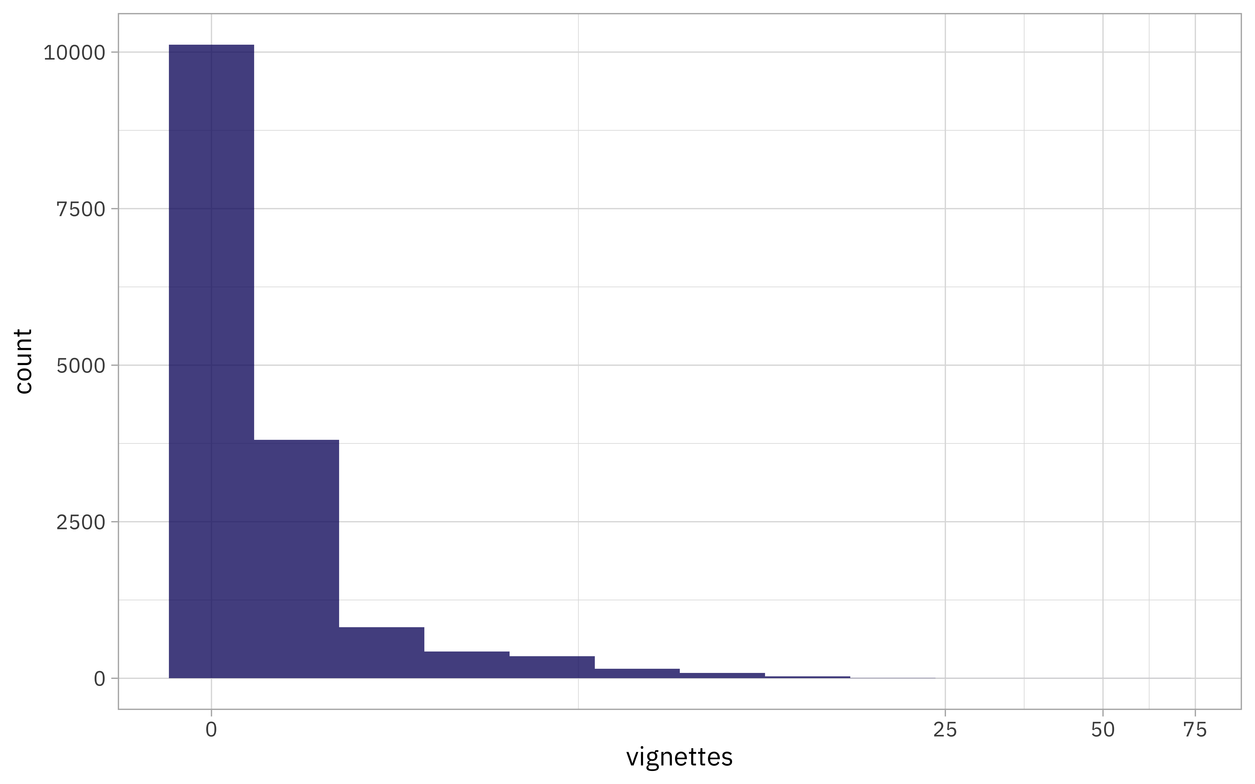
Just a few packages have a ton of vignettes:

vignette_counts %>% filter(vignettes > 20)

## # A tibble: 4 × 4
##   package release_date        releases vignettes
##   <chr>   <dttm>                 <int>     <dbl>
## 1 catdata 2012-02-03 10:29:32        4        45
## 2 fastai  2020-11-05 18:26:03        9        24
## 3 HSAUR3  2014-04-17 10:31:57       11        23
## 4 pla     2015-08-18 21:58:53        2        61

Let’s make one more exploratory plot before creating models.

vignette_counts %>%
  mutate(has_vignette = vignettes > 0) %>%
  ggplot(aes(has_vignette, releases, color = has_vignette, fill = has_vignette)) +
  geom_boxplot(size = 1.5, alpha = 0.2, show.legend = FALSE) +
  scale_y_log10() +
  coord_flip() +
  labs(x = "Has a vignette?")

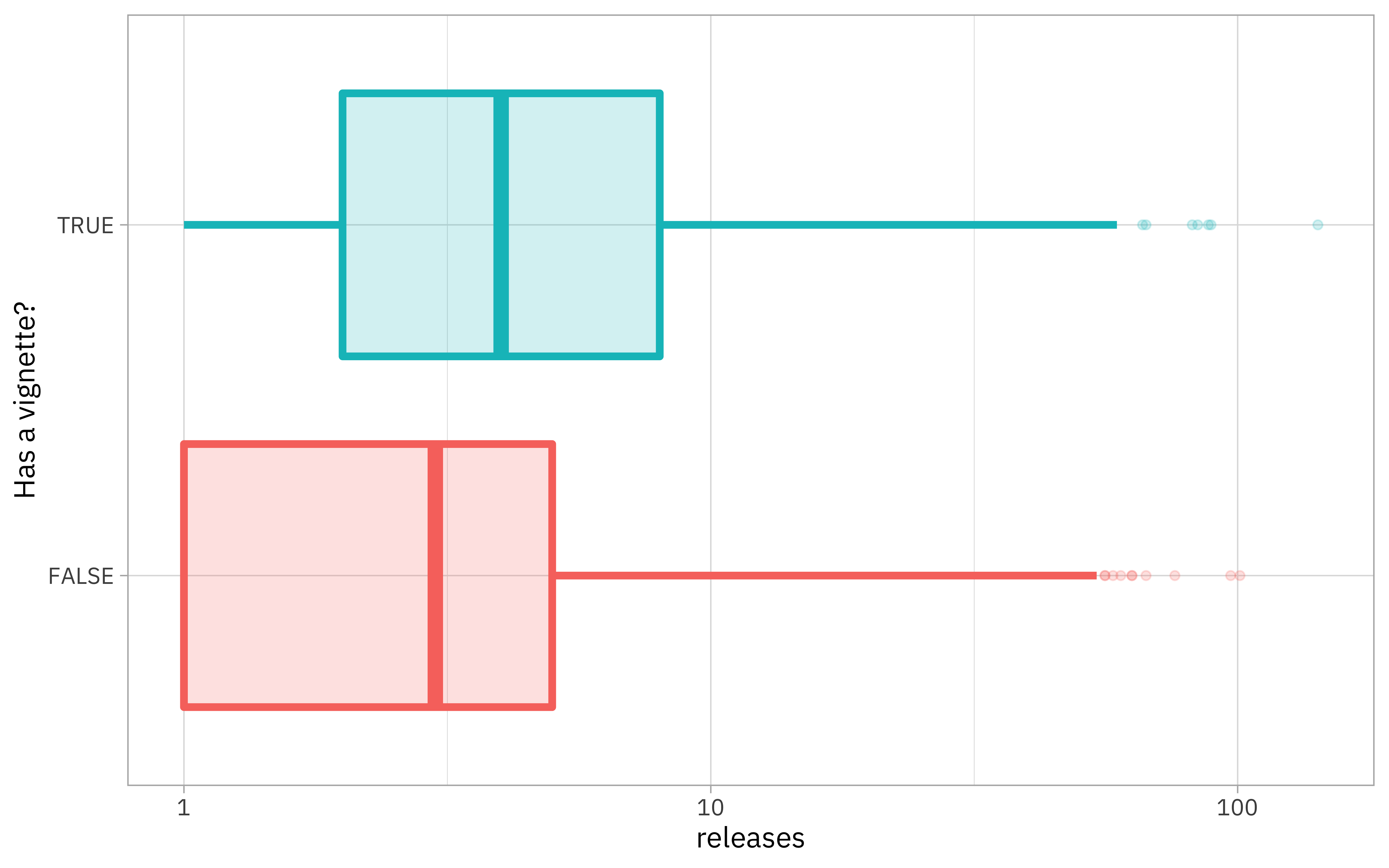
Looks like packages with more releases are more likely to have a vignette.

Using Poisson regression

We have a number of specialized packages, outside the core tidymodels packages, for less general, more specialized data analysis and modeling tasks. One of these is poissonreg, for Poisson regression models such as those we can use with this count data.

library(tidymodels)
library(poissonreg)

poisson_wf <- workflow(vignettes ~ releases, poisson_reg())
fit(poisson_wf, data = vignette_counts)

## ══ Workflow [trained] ══════════════════════════════════════════════════════════
## Preprocessor: Formula
## Model: poisson_reg()
## 
## ── Preprocessor ────────────────────────────────────────────────────────────────
## vignettes ~ releases
## 
## ── Model ───────────────────────────────────────────────────────────────────────
## 
## Call:  stats::glm(formula = ..y ~ ., family = stats::poisson, data = data)
## 
## Coefficients:
## (Intercept)     releases  
##    -0.58265      0.03047  
## 
## Degrees of Freedom: 15793 Total (i.e. Null);  15792 Residual
## Null Deviance:       28880 
## Residual Deviance: 27820     AIC: 41110

This model says that packages with more releases have more vignettes. Since poissonreg is not a core tidymodels package, we need to load it separately via library(poissonreg).

Zero-inflated Poisson: ZIP!!!

A better model for this dataset on R package vignettes might be zero-inflated Poisson, since there are so many zeroes. A ZIP model like this mixes two models, one that generates zeroes and one that models counts with the Poisson distribution. There are two sets of covariates for these two models, that can be different:

• one for the count data
• one for the probability of zeroes

How can we create this kind of model in tidymodels?

zip_spec <- poisson_reg() %>% set_engine("zeroinfl")
zip_wf <- workflow() %>%
  add_variables(outcomes = vignettes, predictors = releases) %>%
  add_model(zip_spec, formula = vignettes ~ releases | releases)

fit(zip_wf, data = vignette_counts)

## ══ Workflow [trained] ══════════════════════════════════════════════════════════
## Preprocessor: Variables
## Model: poisson_reg()
## 
## ── Preprocessor ────────────────────────────────────────────────────────────────
## Outcomes: vignettes
## Predictors: releases
## 
## ── Model ───────────────────────────────────────────────────────────────────────
## 
## Call:
## pscl::zeroinfl(formula = vignettes ~ releases | releases, data = data)
## 
## Count model coefficients (poisson with log link):
## (Intercept)     releases  
##      0.1679       0.0247  
## 
## Zero-inflation model coefficients (binomial with logit link):
## (Intercept)     releases  
##      0.2019      -0.0271

The coefficients here are different than when we didn’t use a ZIP model, but we still see that packages with more releases have more vignettes (and packages with fewer releases are more likely to have zero vignettes).

Notice the formula argument we used in add_model(); this kind of special model formula can be used with a lot of the parsnip-adjacent packages. The formula vignettes ~ releases | releases specifies which columns affect the counts and which affect the model for the probability of zero counts. Here these are the same, but they don’t have to be.

Bootstrap intervals for the coefficients

You can do all the normal things with these models, depending on the purpose of your model. Often these kinds of models are trained to be used in inference, so let’s show how you might determine bootstrap intervals for model coefficients.

First let’s create a set of bootstrap resamples:

folds <- bootstraps(vignette_counts, times = 1000, apparent = TRUE)
folds

## # Bootstrap sampling with apparent sample 
## # A tibble: 1,001 × 2
##    splits               id           
##    <list>               <chr>        
##  1 <split [15794/5840]> Bootstrap0001
##  2 <split [15794/5819]> Bootstrap0002
##  3 <split [15794/5830]> Bootstrap0003
##  4 <split [15794/5858]> Bootstrap0004
##  5 <split [15794/5860]> Bootstrap0005
##  6 <split [15794/5805]> Bootstrap0006
##  7 <split [15794/5875]> Bootstrap0007
##  8 <split [15794/5777]> Bootstrap0008
##  9 <split [15794/5845]> Bootstrap0009
## 10 <split [15794/5752]> Bootstrap0010
## # … with 991 more rows

Now let’s create a little function to get out the coefficients for the probability-of-zero-counts part of our ZIP model. (We could instead or in addition get out the Poisson/count part of the ZIP model.)

get_coefs <- function(x) {
  x %>%
    extract_fit_engine() %>%
    tidy(type = "zero")
}

fit(zip_wf, data = vignette_counts) %>% get_coefs()

## # A tibble: 2 × 6
##   term        type  estimate std.error statistic  p.value
##   <chr>       <chr>    <dbl>     <dbl>     <dbl>    <dbl>
## 1 (Intercept) zero    0.202    0.0310       6.51 7.63e-11
## 2 releases    zero   -0.0271   0.00322     -8.41 3.94e-17

We can now take this function and use it for all of our bootstrap resamples with our ZIP model.

ctrl <- control_resamples(extract = get_coefs)

doParallel::registerDoParallel()
set.seed(123)
zip_res <- fit_resamples(zip_wf, folds, control = ctrl)
zip_res

## # Resampling results
## # Bootstrap sampling with apparent sample 
## # A tibble: 1,001 × 5
##    splits                id            .metrics         .notes   .extracts
##    <list>                <chr>         <list>           <list>   <list>   
##  1 <split [15794/15794]> Apparent      <tibble [2 × 4]> <tibble> <tibble> 
##  2 <split [15794/5840]>  Bootstrap0001 <tibble [2 × 4]> <tibble> <tibble> 
##  3 <split [15794/5819]>  Bootstrap0002 <tibble [2 × 4]> <tibble> <tibble> 
##  4 <split [15794/5830]>  Bootstrap0003 <tibble [2 × 4]> <tibble> <tibble> 
##  5 <split [15794/5858]>  Bootstrap0004 <tibble [2 × 4]> <tibble> <tibble> 
##  6 <split [15794/5860]>  Bootstrap0005 <tibble [2 × 4]> <tibble> <tibble> 
##  7 <split [15794/5805]>  Bootstrap0006 <tibble [2 × 4]> <tibble> <tibble> 
##  8 <split [15794/5875]>  Bootstrap0007 <tibble [2 × 4]> <tibble> <tibble> 
##  9 <split [15794/5777]>  Bootstrap0008 <tibble [2 × 4]> <tibble> <tibble> 
## 10 <split [15794/5845]>  Bootstrap0009 <tibble [2 × 4]> <tibble> <tibble> 
## # … with 991 more rows

What is in that .extracts column?

zip_res$.extracts[[33]]

## # A tibble: 1 × 2
##   .extracts        .config             
##   <list>           <chr>               
## 1 <tibble [2 × 6]> Preprocessor1_Model1

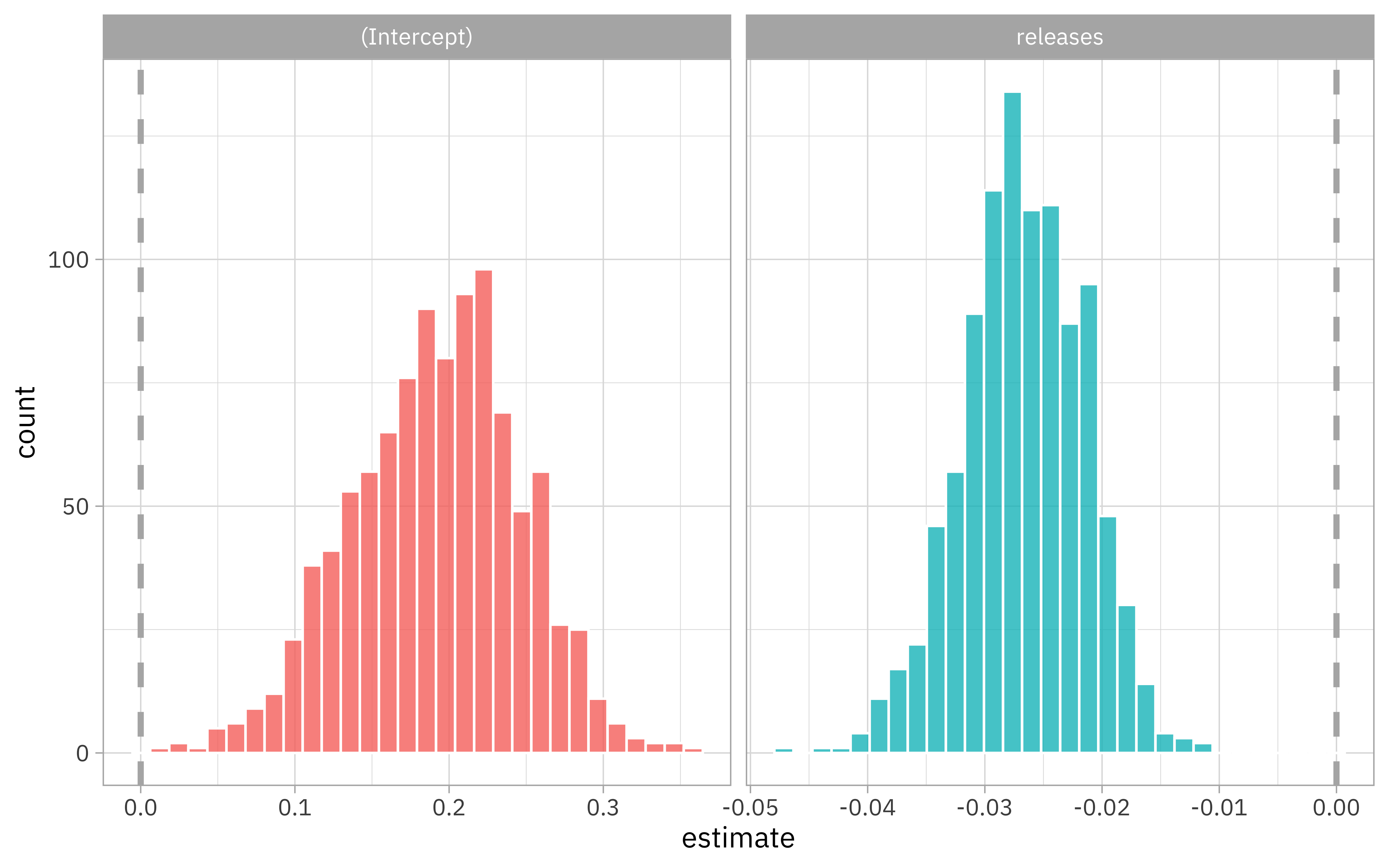
We can use tidyr to get those out, and then we can visualize the bootstrap intervals.

zip_res %>%
  select(id, .extracts) %>%
  unnest(.extracts) %>%
  unnest(.extracts) %>%
  ggplot(aes(x = estimate, fill = term)) +
  geom_histogram(color = "white", alpha = 0.8, show.legend = FALSE) +
  facet_wrap(~term, scales = "free_x") +
  geom_vline(xintercept = 0, lty = 2, size = 1.2, color = "gray70")