Inference for #TidyTuesday aircraft and rank of Tuskegee airmen

This is the latest in my series of screencasts demonstrating how to use the tidymodels packages. Instead of predictive modeling, this screencast focuses on statistical inference using one of the tidymodels package, infer. We are celebrating Black History Month by learning more from the #TidyTuesday dataset on the Tuskegee airmen. ✈️

Here is the code I used in the video, for those who prefer reading instead of or in addition to video.

Explore data

Our statistical analysis goal is to understand the relationship between aircraft flown and rank at graduation for the Tuskegee airmen. What kind of aircraft did the airmen pilot?

library(tidyverse)

airmen_raw <- read_csv("https://raw.githubusercontent.com/rfordatascience/tidytuesday/master/data/2022/2022-02-08/airmen.csv")

airmen_raw %>% count(pilot_type)

## # A tibble: 5 × 2
##   pilot_type        n
##   <chr>         <int>
## 1 Liaison pilot    50
## 2 Liason pilot      1
## 3 Service pilot    11
## 4 Single engine   697
## 5 Twin engine     247

Let’s fix the spelling error and visualize the relationship between the type of aircraft piloted and the rank at graduation.

airmen <-
  airmen_raw %>%
  mutate(pilot_type = str_replace(pilot_type, "Liason", "Liaison"))

airmen %>%
  ggplot(aes(pilot_type, fill = rank_at_graduation)) +
  geom_bar(stat = "count")

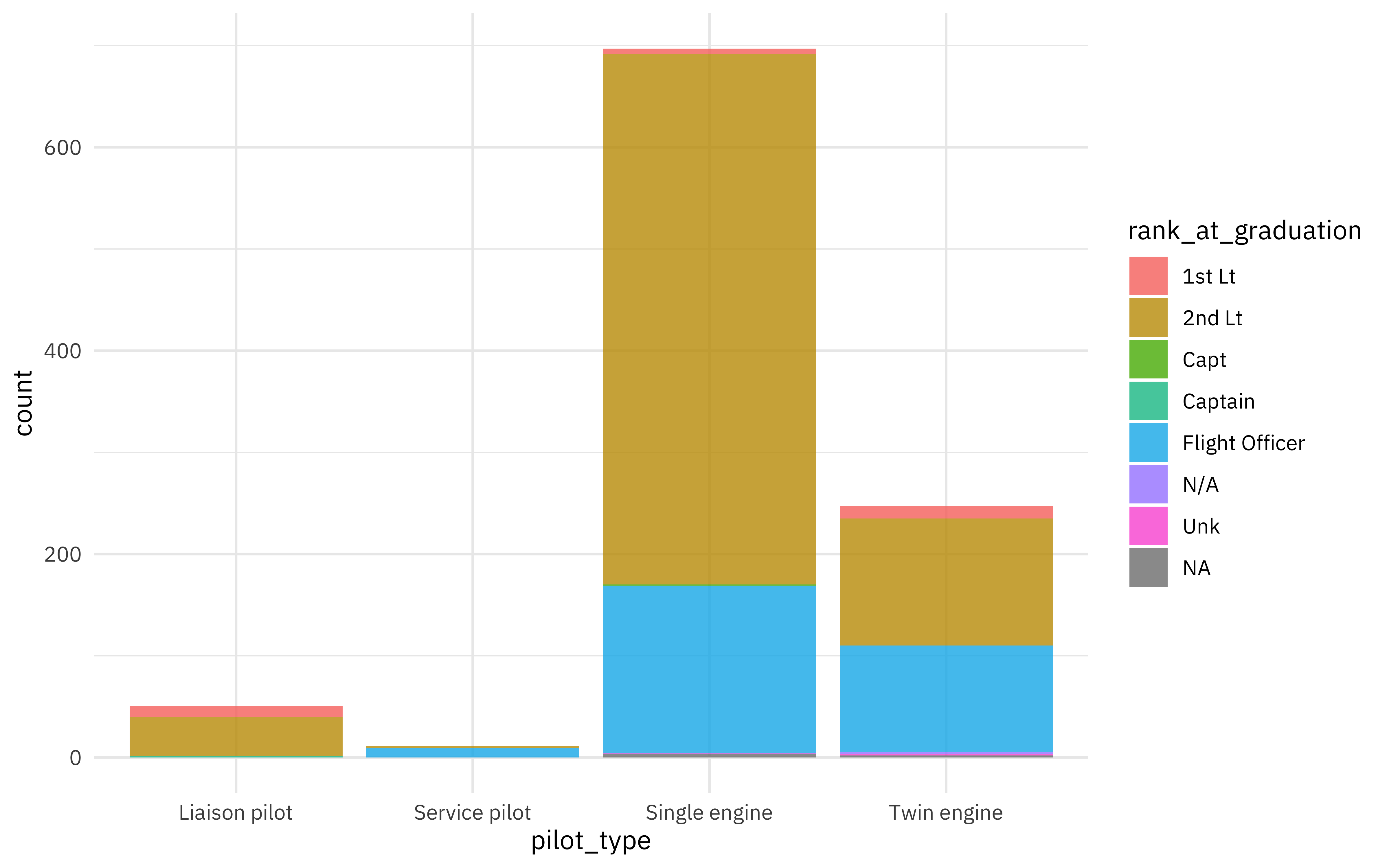
A lieutenant is a higher rank than a flight officer. The categories with the most airmen are single and twin engine aircraft, as well as flight officers and second lieutenants, so let’s focus on those.

Using infer

The infer package provides an expressive grammar for statistical inference. We start out by using specify() to declare our response and explanatory variables. Then we can start generating resamples, like bootstrap resamples and permutations.

library(infer)

aircraft <- c("Single engine", "Twin engine")
ranks <- c("Flight Officer", "2nd Lt")

pilot_vs_rank <-
  airmen %>%
  filter(pilot_type %in% aircraft, rank_at_graduation %in% ranks) %>%
  specify(pilot_type ~ rank_at_graduation, success = "Twin engine")

set.seed(123)
bootstrapped <-
  pilot_vs_rank %>%
  generate(reps = 1000, type = "bootstrap")

bootstrapped

## Response: pilot_type (factor)
## Explanatory: rank_at_graduation (factor)
## # A tibble: 917,000 × 3
## # Groups:   replicate [1,000]
##    replicate pilot_type    rank_at_graduation
##        <int> <fct>         <fct>             
##  1         1 Single engine 2nd Lt            
##  2         1 Single engine 2nd Lt            
##  3         1 Twin engine   Flight Officer    
##  4         1 Single engine 2nd Lt            
##  5         1 Single engine 2nd Lt            
##  6         1 Twin engine   Flight Officer    
##  7         1 Single engine 2nd Lt            
##  8         1 Single engine 2nd Lt            
##  9         1 Twin engine   Flight Officer    
## 10         1 Twin engine   Flight Officer    
## # … with 916,990 more rows

set.seed(234)
permuted <-
  pilot_vs_rank %>%
  hypothesize(null = "independence") %>%
  generate(reps = 1000, type = "permute")

permuted

## Response: pilot_type (factor)
## Explanatory: rank_at_graduation (factor)
## Null Hypothesis: independence
## # A tibble: 917,000 × 3
## # Groups:   replicate [1,000]
##    pilot_type    rank_at_graduation replicate
##    <fct>         <fct>                  <int>
##  1 Single engine 2nd Lt                     1
##  2 Single engine 2nd Lt                     1
##  3 Single engine 2nd Lt                     1
##  4 Single engine 2nd Lt                     1
##  5 Single engine 2nd Lt                     1
##  6 Single engine 2nd Lt                     1
##  7 Single engine 2nd Lt                     1
##  8 Single engine 2nd Lt                     1
##  9 Single engine 2nd Lt                     1
## 10 Single engine 2nd Lt                     1
## # … with 916,990 more rows

Chi-squared statistic

Now that we have different kinds of resampled datasets, we can compute some statistics. Let’s start with the chi-squared statistic; this is a number that tells us how much difference exists between our observed counts (aircraft types, ranks at graduation) and the counts we would expect if there were no relationship in the population of airmen.

We can compute the chi-squared statistic in our real sample:

observed <-
  pilot_vs_rank %>%
  calculate(stat = "chisq", order = ranks)

observed

## Response: pilot_type (factor)
## Explanatory: rank_at_graduation (factor)
## # A tibble: 1 × 1
##    stat
##   <dbl>
## 1  37.8

That seems big (indicating that aircraft type and rank are related) but how do we know if it’s meaningful for our dataset? I mean, we are pretty sure it is, based on our EDA, but how can we check? We can compute the statistic for our bootstrapped resamples and find a confidence interval:

airmen_chisq <-
  bootstrapped %>%
  calculate(stat = "chisq", order = ranks)

get_ci(airmen_chisq)

## # A tibble: 1 × 2
##   lower_ci upper_ci
##      <dbl>    <dbl>
## 1     16.7     64.1

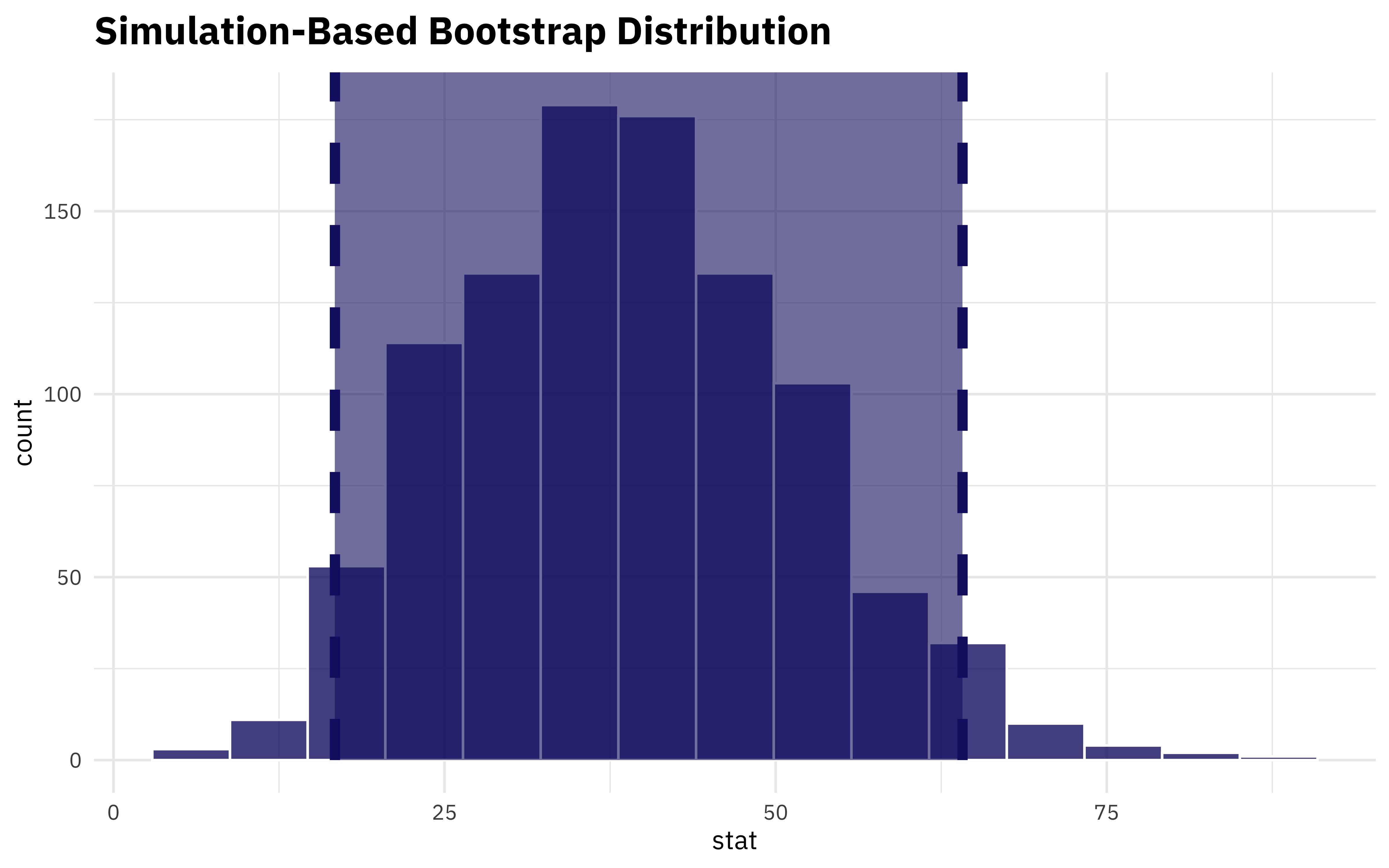
We can also visualize the distribution together with the confidence interval.

visualize(airmen_chisq) +
  shade_ci(
    endpoints = get_ci(airmen_chisq),
    fill = "midnightblue",
    color = "midnightblue",
    lty = 2
  )

What if we want to understand how extreme this value is? We can compute the statistic for the permuted data (which breaks the relationship between aircraft and rank) and see how our real observed statistic compares.

permuted %>%
  calculate(stat = "chisq", order = ranks) %>%
  visualize() +
  shade_p_value(obs_stat = observed, direction = NULL, color = "gray40", lty = 2)

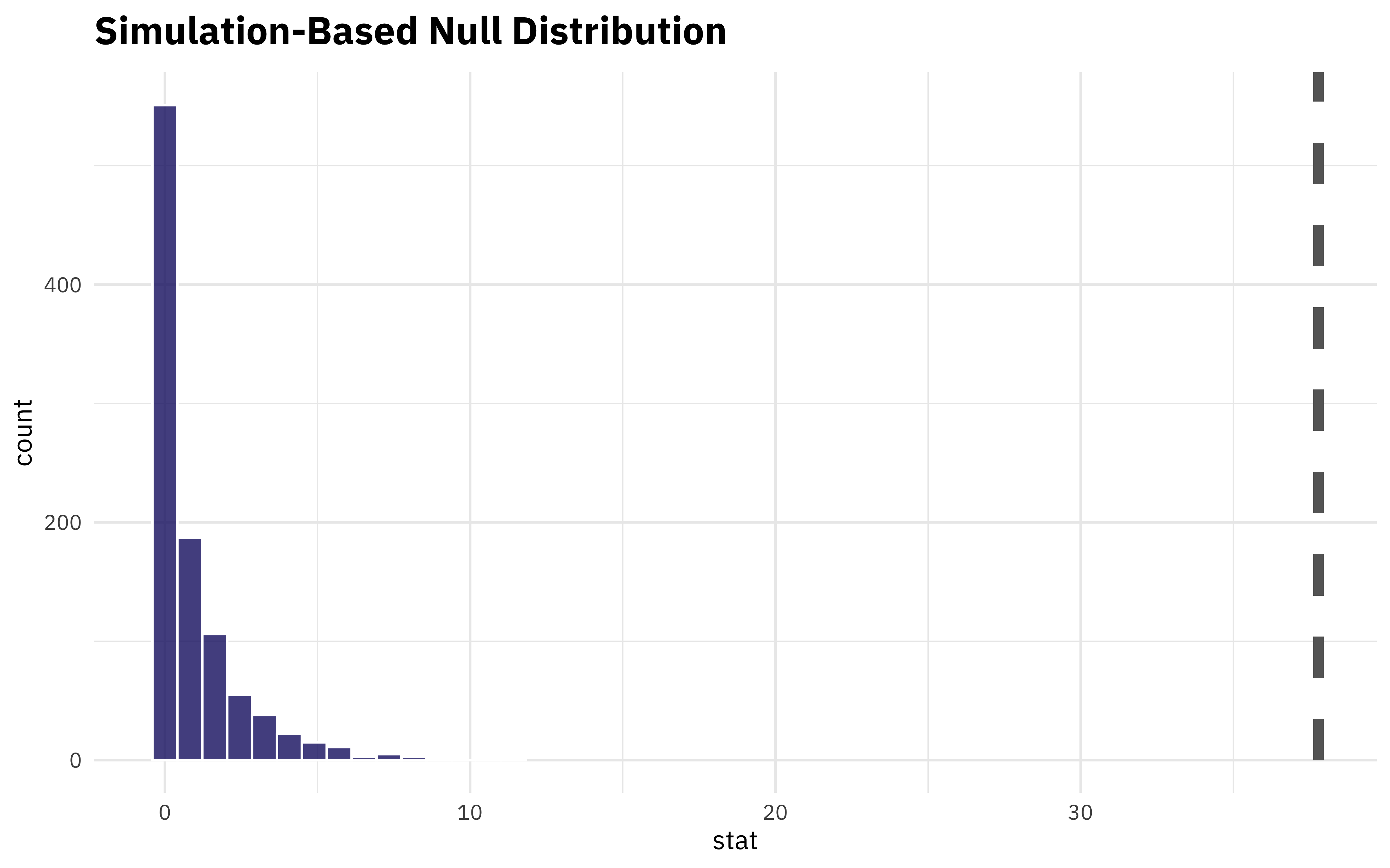
Well, the p-value for that would be tiny! Using resampling and simulation instead of a regular chisq.test() with a p-value can help us understand the statistical relationships here.

Odds ratio

I’ll be honest that the chi-squared statistic isn’t one I have a ton of intuition about. Odds ratios, on the other hand, make a lot of sense to me. One great thing about infer is that we can switch out the stat we compute and do any of the previous steps again. Let’s make a visualization of the bootstrapped odds ratio distribution.

odds_desc <- paste(
  "Flight officers were more likely to pilot twin engine aircraft",
  "2nd Lts were more likely to pilot single engine aircraft",
  sep = "\n"
)

bootstrapped %>%
  calculate(stat = "odds ratio", order = ranks) %>%
  visualize() +
  labs(
    title = "Bootstrap distribution of Tuskegee airmen's rank by aircraft type",
    subtitle = odds_desc,
    x = "Odds ratio of twin vs. single engine (for flight officers compared to 2nd Lt)"
  )

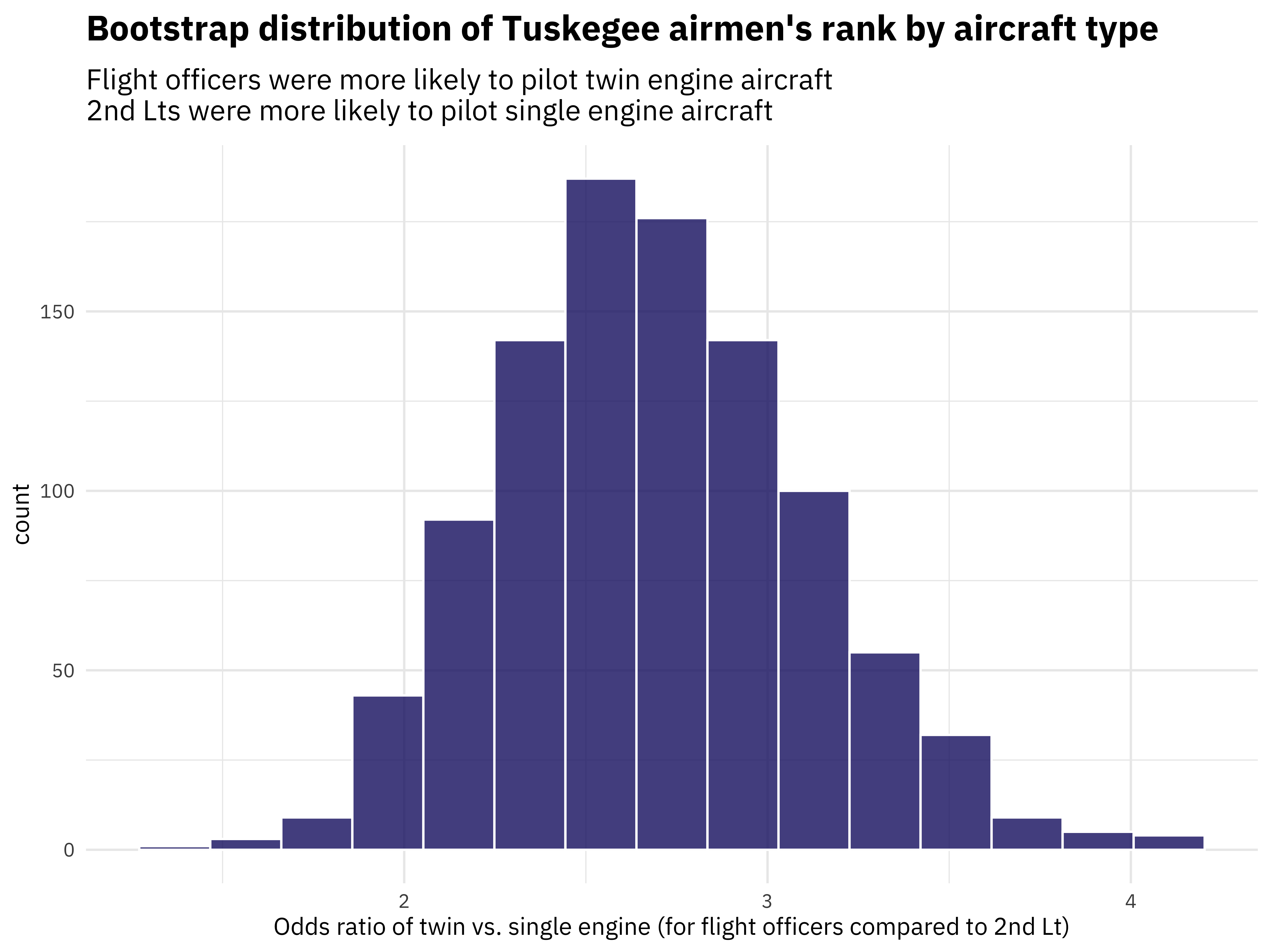
When comparing twin and single engines, flight officers are 2 or 3 times more likely to pilot a twin engine than a second lieutenant.