Tune xgboost models with early stopping to predict shelter animal status
By Julia Silge in rstats tidymodels
August 7, 2021
This is the latest in my series of screencasts demonstrating how to use the tidymodels packages, from just getting started to tuning more complex models. I participated in this week’s episode of the SLICED playoffs, a competitive data science streaming show, where we competed to predict the status of shelter animals. 🐱 I used xgboost’s early stopping feature as I competed, so let’s walk through how and when to try that out!
Here is the code I used in the video, for those who prefer reading instead of or in addition to video.
Explore data
Our modeling goal is to predict
the outcome for shelter animals (adoption, transfer, or no outcome) given features about the animal and event. The main data set provided is in a CSV file called training.csv.
library(tidyverse)
train_raw <- read_csv("train.csv")
You can watch this week’s full episode of SLICED to see lots of exploratory data analysis and visualization of this dataset, but let’s just make a few plots to understand it better.
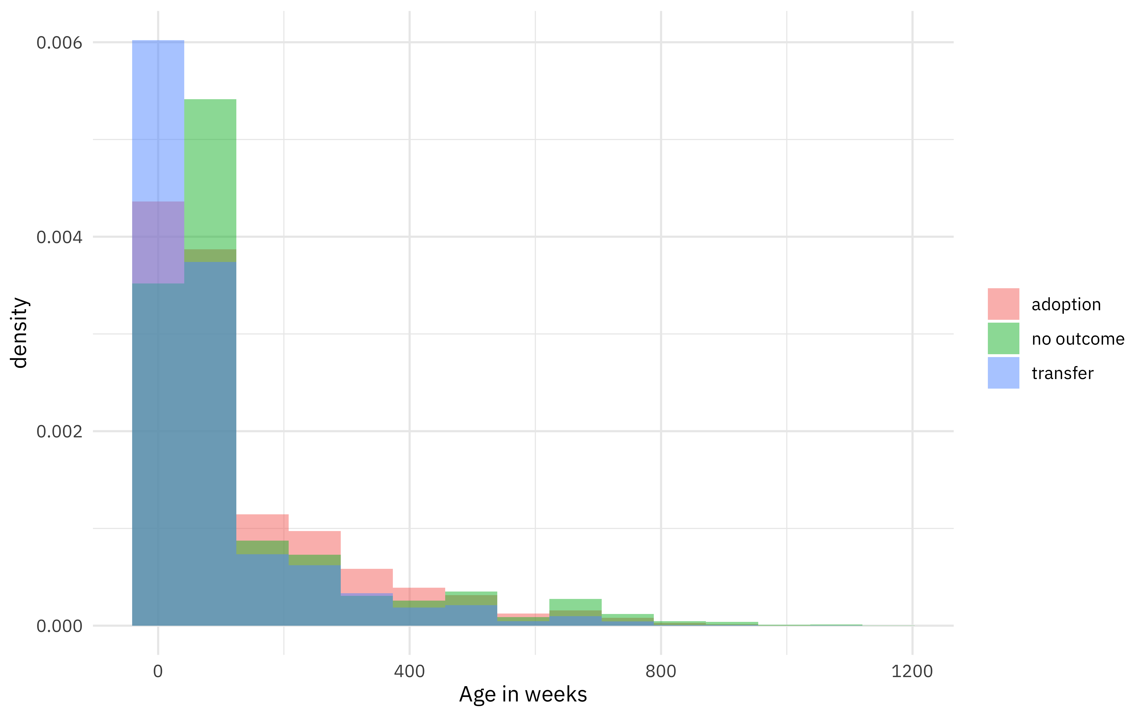
How are outcomes distributed for animals of different ages?
library(lubridate)

train_raw %>%
  mutate(
    age_upon_outcome = as.period(as.Date(datetime) - date_of_birth),
    age_upon_outcome = time_length(age_upon_outcome, unit = "weeks")
  ) %>%
  ggplot(aes(age_upon_outcome, after_stat(density), fill = outcome_type)) +
  geom_histogram(bins = 15, alpha = 0.5, position = "identity") +
  labs(x = "Age in weeks", fill = NULL)
How does adoption rate change with day of the week and week of the year?
train_raw %>%
  mutate(outcome_type = outcome_type == "adoption") %>%
  group_by(
    week = week(datetime),
    wday = wday(datetime)
  ) %>%
  summarise(outcome_type = mean(outcome_type)) %>%
  ggplot(aes(week, wday, fill = outcome_type)) +
  geom_tile(alpha = 0.8) +
  scale_fill_viridis_c(labels = scales::percent) +
  labs(fill = "% adopted", x = "week of the year", y = "week day")
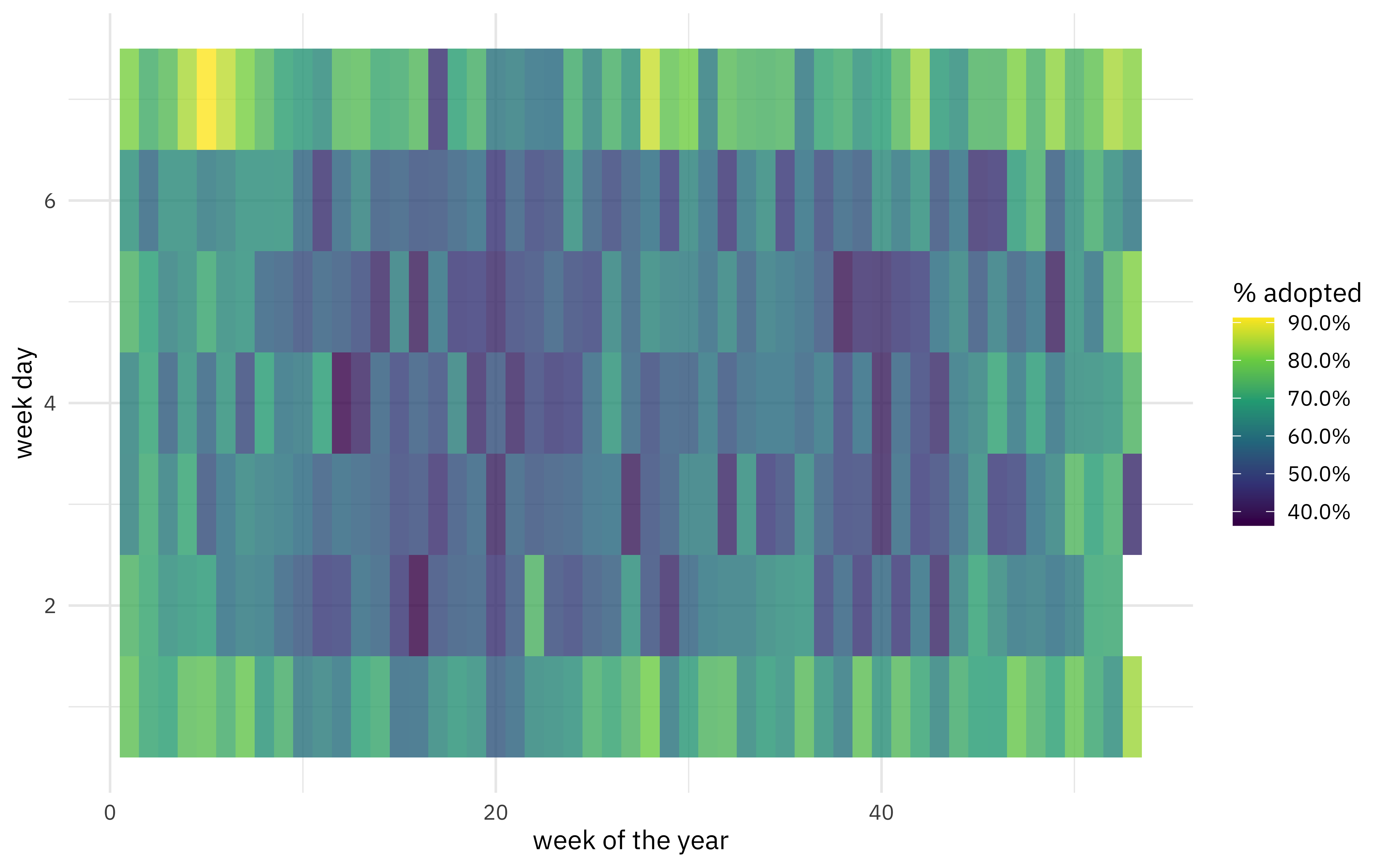
Notice the difference on weekends vs. weekdays especially!
There is certainly lots more to explore (including, for example, learning about the names of the animals, something I spent a good bit of time on during the competition), but let’s move on to modeling.
Build a model
Let’s start our modeling by setting up our “data budget,” as well as the metrics (this challenge was evaluate on multiclass log loss).
library(tidymodels)

set.seed(123)
shelter_split <- train_raw %>%
  mutate(
    age_upon_outcome = as.period(as.Date(datetime) - date_of_birth),
    age_upon_outcome = time_length(age_upon_outcome, unit = "weeks")
  ) %>%
  initial_split(strata = outcome_type)

shelter_train <- training(shelter_split)
shelter_test <- testing(shelter_split)
shelter_metrics <- metric_set(accuracy, roc_auc, mn_log_loss)

set.seed(234)
shelter_folds <- vfold_cv(shelter_train, strata = outcome_type)
shelter_folds
## #  10-fold cross-validation using stratification
## # A tibble: 10 × 2
##    splits               id
##    <list>               <chr>
##  1 <split [36724/4081]> Fold01
##  2 <split [36724/4081]> Fold02
##  3 <split [36724/4081]> Fold03
##  4 <split [36724/4081]> Fold04
##  5 <split [36724/4081]> Fold05
##  6 <split [36725/4080]> Fold06
##  7 <split [36725/4080]> Fold07
##  8 <split [36725/4080]> Fold08
##  9 <split [36725/4080]> Fold09
## 10 <split [36725/4080]> Fold10
For feature engineering, let’s concentrate on just a handful of predictors, like when the event (adoption, transfer, or “no outcome”) was recorded and features of the animal itself like age, sex, type, etc.
shelter_rec <- recipe(outcome_type ~ age_upon_outcome + animal_type +
  datetime + sex + spay_neuter,
data = shelter_train
) %>%
  step_date(datetime, features = c("year", "week", "dow"), keep_original_cols = FALSE) %>%
  step_dummy(all_nominal_predictors(), one_hot = TRUE) %>%
  step_zv(all_predictors())

## we can `prep()` just to check that it works
prep(shelter_rec)
## Data Recipe
##
## Inputs:
##
##       role #variables
##    outcome          1
##  predictor          5
##
## Training data contained 40805 data points and no missing data.
##
## Operations:
##
## Date features from datetime [trained]
## Dummy variables from animal_type, sex, spay_neuter, datetime_dow [trained]
## Zero variance filter removed no terms [trained]
Now let’s create a tunable xgboost model specification. This is where
early stopping comes in; we will keep the number of trees as a constant (and not too terribly high), set stop_iter (the early stopping parameter) to tune(), and then tune a few other parameters. Notice that we need to set a validation set (a proportion of each analysis set, actually) to hold back to use for deciding when to stop.
We can also create a custom stopping_grid to specific what parameters I want to try out.
stopping_spec <-
  boost_tree(
    trees = 500,
    mtry = tune(),
    learn_rate = tune(),
    stop_iter = tune()
  ) %>%
  set_engine("xgboost", validation = 0.2) %>%
  set_mode("classification")

stopping_grid <-
  grid_latin_hypercube(
    mtry(range = c(5L, 20L)), ## depends on number of columns in data
    learn_rate(range = c(-5, -1)), ## keep pretty big
    stop_iter(range = c(10L, 50L)), ## bigger than default
    size = 10
  )
Now we can put these together in a workflow and tune across the grid of parameters and our resamples.
early_stop_wf <- workflow(shelter_rec, stopping_spec)

doParallel::registerDoParallel()
set.seed(345)
stopping_rs <- tune_grid(
  early_stop_wf,
  shelter_folds,
  grid = stopping_grid,
  metrics = shelter_metrics
)
We did it!
Evaluate results
How did these results turn out? We can visualize them.
autoplot(stopping_rs) + theme_light(base_family = "IBMPlexSans")
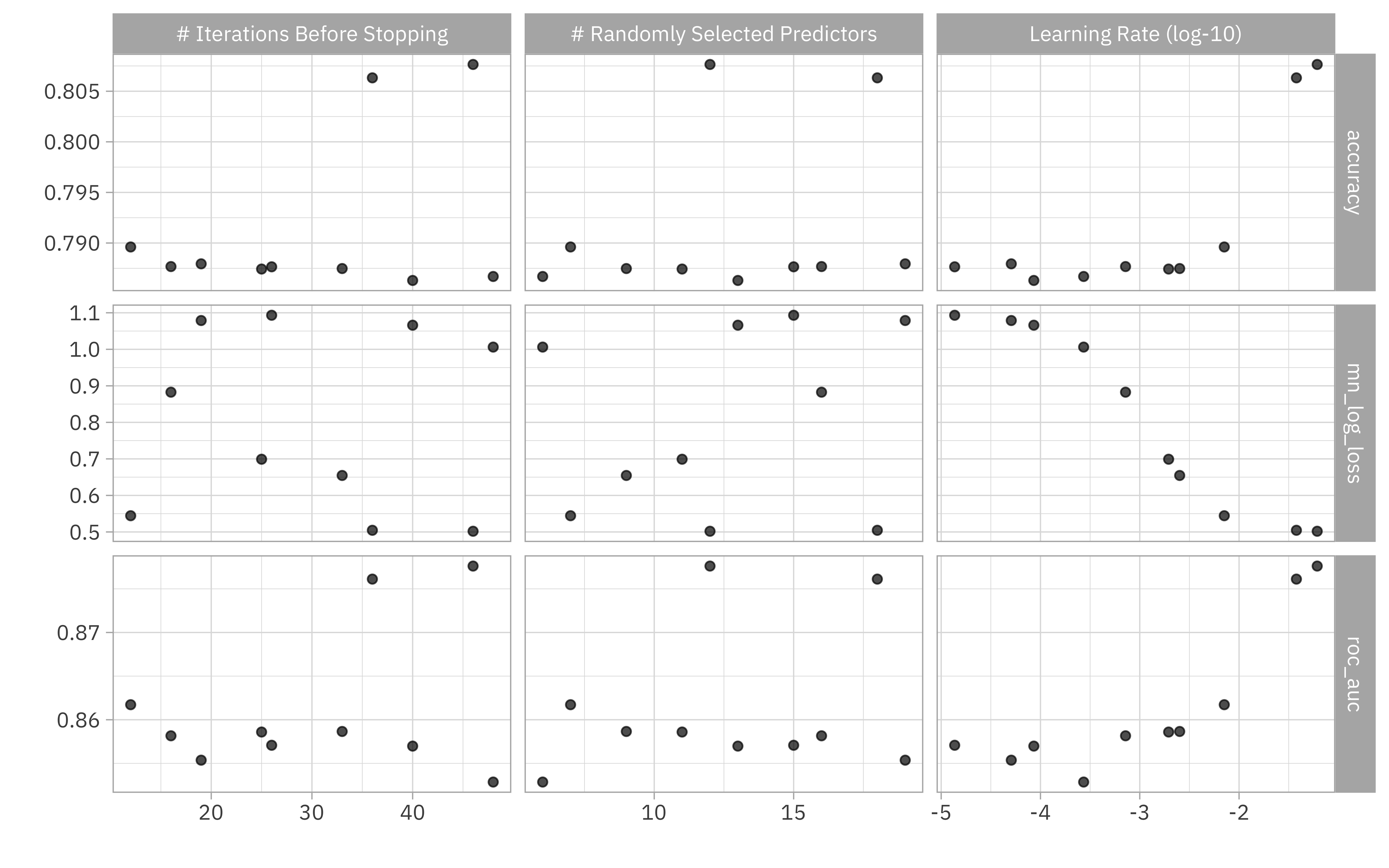
Or we can look at the top results manually.
show_best(stopping_rs, metric = "mn_log_loss")
## # A tibble: 5 × 9
##    mtry learn_rate stop_iter .metric     .estimator  mean     n std_err .config
##   <int>      <dbl>     <int> <chr>       <chr>      <dbl> <int>   <dbl> <chr>
## 1    12    0.0612         46 mn_log_loss multiclass 0.502    10 0.00319 Preproc…
## 2    18    0.0378         36 mn_log_loss multiclass 0.505    10 0.00279 Preproc…
## 3     7    0.00710        12 mn_log_loss multiclass 0.544    10 0.00246 Preproc…
## 4     9    0.00252        33 mn_log_loss multiclass 0.655    10 0.00145 Preproc…
## 5    11    0.00195        25 mn_log_loss multiclass 0.699    10 0.00122 Preproc…
Let’s use last_fit() to fit one final time to the training data and evaluate one final time on the testing data, with the numerically optimal result from stopping_rs.
stopping_fit <- early_stop_wf %>%
  finalize_workflow(select_best(stopping_rs, "mn_log_loss")) %>%
  last_fit(shelter_split)

stopping_fit
## # Resampling results
## # Manual resampling
## # A tibble: 1 × 6
##   splits                id               .metrics  .notes .predictions .workflow
##   <list>                <chr>            <list>    <list> <list>       <list>
## 1 <split [40805/13603]> train/test split <tibble … <tibb… <tibble [13… <workflo…
How did this model perform on the testing data, that was not used in tuning/training?
collect_metrics(stopping_fit)
## # A tibble: 2 × 4
##   .metric  .estimator .estimate .config
##   <chr>    <chr>          <dbl> <chr>
## 1 accuracy multiclass     0.807 Preprocessor1_Model1
## 2 roc_auc  hand_till      0.877 Preprocessor1_Model1
This result is pretty good for a single model; we would expect to do better by incorporating the breed information, perhaps the presence/absence of a name, or moving to an ensembled model.
What features are most important for this xgboost model?
library(vip)

## use this fitted workflow `extract_workflow(stopping_fit)` to predict on new data
extract_workflow(stopping_fit) %>%
  extract_fit_parsnip() %>%
  vip(num_features = 15, geom = "point")
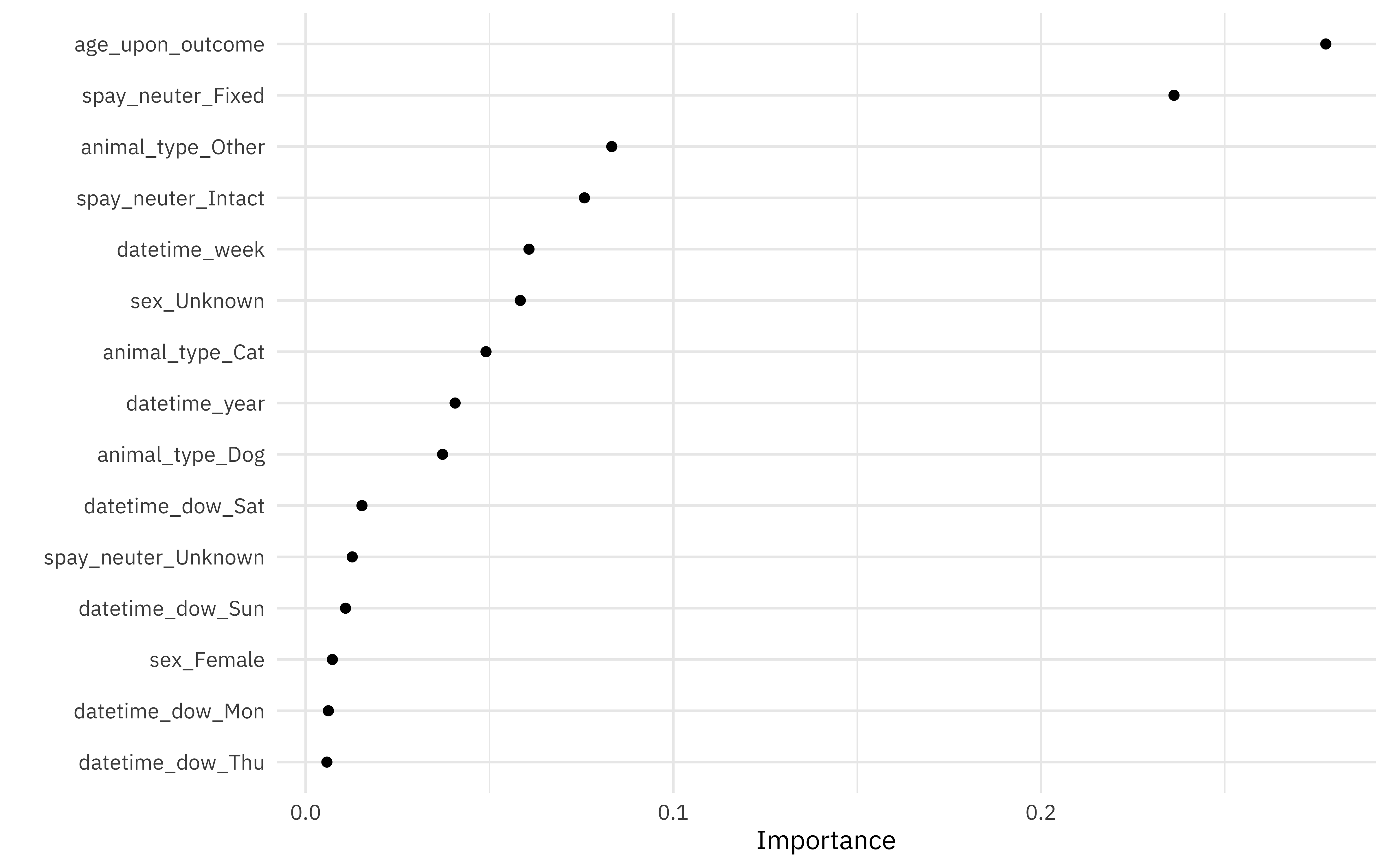
Age, spay/neuter status, animal type, and seasonal information like week of the year or day of the week are important for this model.
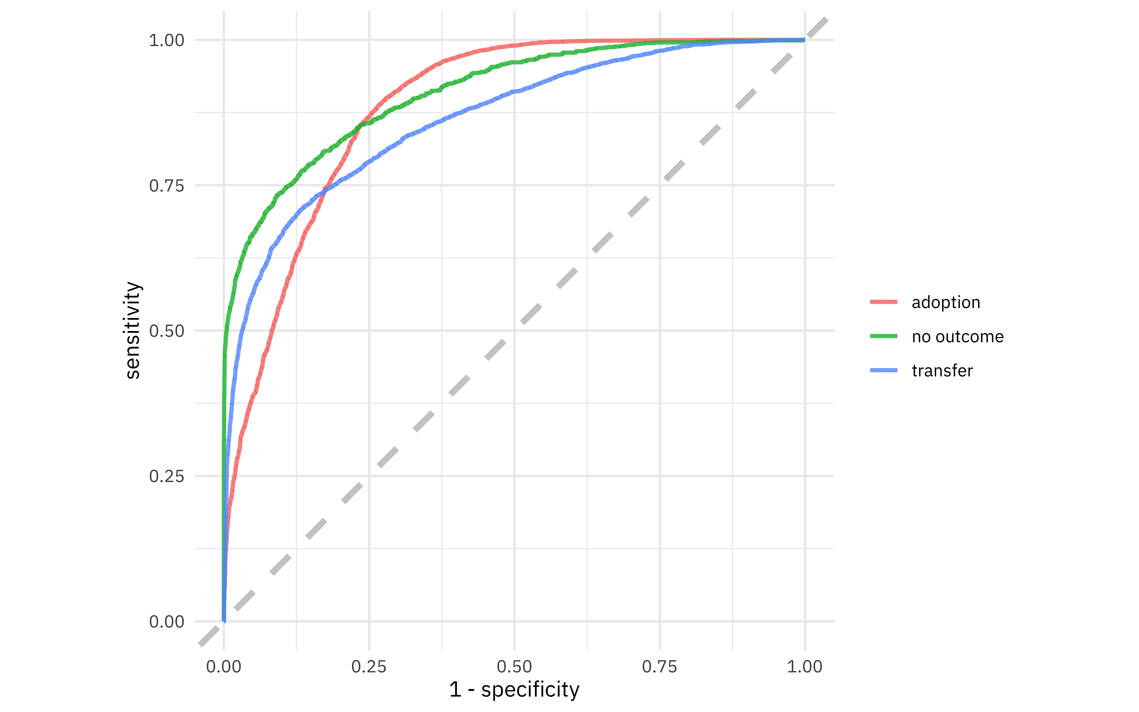
We can collect the predictions on the testing set and do whatever we want, like create an ROC curve.
collect_predictions(stopping_fit) %>%
  roc_curve(outcome_type, .pred_adoption:.pred_transfer) %>%
  ggplot(aes(1 - specificity, sensitivity, color = .level)) +
  geom_abline(lty = 2, color = "gray80", size = 1.5) +
  geom_path(alpha = 0.8, size = 1) +
  coord_equal() +
  labs(color = NULL)
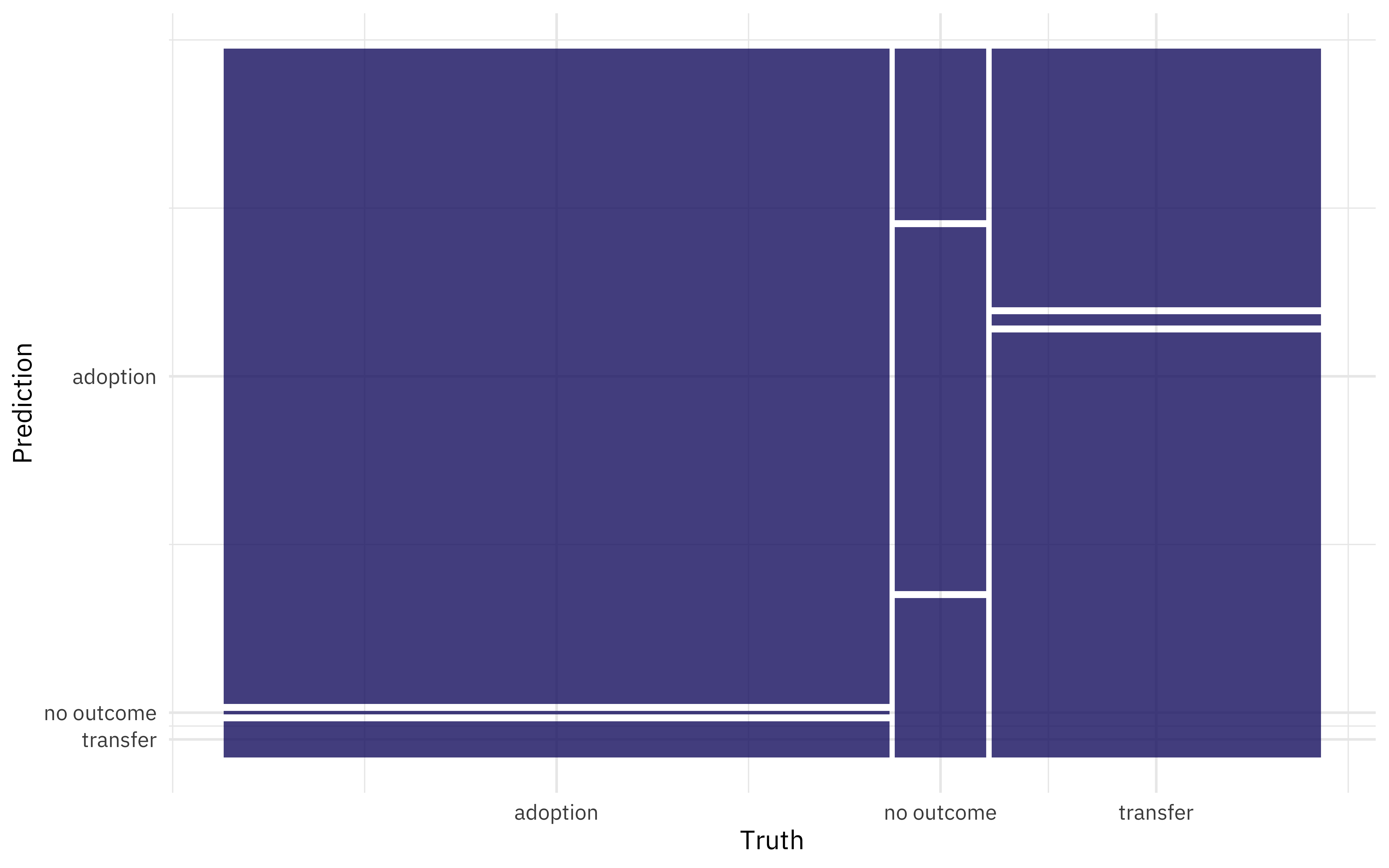
We can also look at a confusion matrix.
collect_predictions(stopping_fit) %>%
  conf_mat(outcome_type, .pred_class) %>%
  autoplot()
Early stopping is a great option when you have plenty of data and don’t want to overfit your boosted trees! I will be back on SLICED for the final four next Tuesday, and I plan to use early stopping again because it is a good fit for this kind of situation.
- Posted on:
- August 7, 2021
- Length:
- 6 minute read, 1218 words
- Categories:
- rstats tidymodels
- Tags:
- rstats tidymodels