The game is afoot! Topic modeling of Sherlock Holmes stories
By Julia Silge
January 25, 2018
In a recent release of tidytext, we added tidiers and support for building Structural Topic Models from the stm package. This is my current favorite implementation of topic modeling in R, so let’s walk through an example of how to get started with this kind of modeling, using The Adventures of Sherlock Holmes.
You can watch along as I demonstrate how to start with the raw text of these short stories, prepare the data, and then implement topic modeling in this video tutorial! 🎉🎉🎉
In the video, I am working on IBM Cloud with IBM’s environment for data scientists, the Data Science Experience. I worked in a browser and my code, packages, plots, etc all lived in this cloud environment, instead of locally on my own computer.
Let’s walk through the code again in more detail, or if you are not in a video watching mood!
First up, let’s download the text of this collection of short stories from Project Gutenberg using the gutenbergr package. Then, let’s do some data manipulation to prepare this text. We can create a new column story that keeps track of which of the twelve short stories each line of text comes from, and remove the preliminary material that comes before the first story actually starts.
library(tidyverse)
library(gutenbergr)

sherlock_raw <- gutenberg_download(1661)

sherlock <- sherlock_raw %>%
    mutate(story = ifelse(str_detect(text, "ADVENTURE"),
                          text,
                          NA)) %>%
    fill(story) %>%
    filter(story != "THE ADVENTURES OF SHERLOCK HOLMES") %>%
    mutate(story = factor(story, levels = unique(story)))

sherlock
## # A tibble: 12,624 x 3
## gutenberg_id
## <int>
## 1 1661
## 2 1661
## 3 1661
## 4 1661
## 5 1661
## 6 1661
## 7 1661
## 8 1661
## 9 1661
## 10 1661
## text story
## <chr> <fct>
## 1 ADVENTURE I. A SCANDAL IN BOHEMIA ADVENTURE I. A SCANDA…
## 2 "" ADVENTURE I. A SCANDA…
## 3 I. ADVENTURE I. A SCANDA…
## 4 "" ADVENTURE I. A SCANDA…
## 5 To Sherlock Holmes she is always THE woman… ADVENTURE I. A SCANDA…
## 6 him mention her under any other name. In h… ADVENTURE I. A SCANDA…
## 7 and predominates the whole of her sex. It … ADVENTURE I. A SCANDA…
## 8 any emotion akin to love for Irene Adler. … ADVENTURE I. A SCANDA…
## 9 one particularly, were abhorrent to his co… ADVENTURE I. A SCANDA…
## 10 admirably balanced mind. He was, I take it… ADVENTURE I. A SCANDA…
## # ... with 12,614 more rowsNext, let’s transform this text data into a tidy data structure using unnest_tokens(). We can also remove stop words at this point because they will not do us any favors during the topic modeling process. Using the stop_words dataset as a whole removes a LOT of stop words; you can be more discriminating and choose specific sets of stop words if appropriate for your purpose. Let’s also remove the word “holmes” because it is so common and used neutrally in all twelve stories.
library(tidytext)

tidy_sherlock <- sherlock %>%
    mutate(line = row_number()) %>%
    unnest_tokens(word, text) %>%
    anti_join(stop_words) %>%
    filter(word != "holmes")

tidy_sherlock %>%
    count(word, sort = TRUE)
## # A tibble: 7,437 x 2
## word n
## <chr> <int>
## 1 time 151
## 2 door 144
## 3 matter 125
## 4 house 123
## 5 hand 120
## 6 night 114
## 7 heard 113
## 8 found 108
## 9 day 106
## 10 morning 102
## # ... with 7,427 more rowsWhat are the highest tf-idf words in these twelve stories? The statistic tf-idf identifies words that are important to a document in a collection of documents; in this case, we’ll see which words are important in one of the stories compared to the others.
library(drlib)

sherlock_tf_idf <- tidy_sherlock %>%
    count(story, word, sort = TRUE) %>%
    bind_tf_idf(word, story, n) %>%
    arrange(-tf_idf) %>%
    group_by(story) %>%
    top_n(10) %>%
    ungroup

sherlock_tf_idf %>%
    mutate(word = reorder_within(word, tf_idf, story)) %>%
    ggplot(aes(word, tf_idf, fill = story)) +
    geom_col(alpha = 0.8, show.legend = FALSE) +
    facet_wrap(~ story, scales = "free", ncol = 3) +
    scale_x_reordered() +
    coord_flip() +
    theme(strip.text=element_text(size=11)) +
    labs(x = NULL, y = "tf-idf",
         title = "Highest tf-idf words in Sherlock Holmes short stories",
         subtitle = "Individual stories focus on different characters and narrative elements")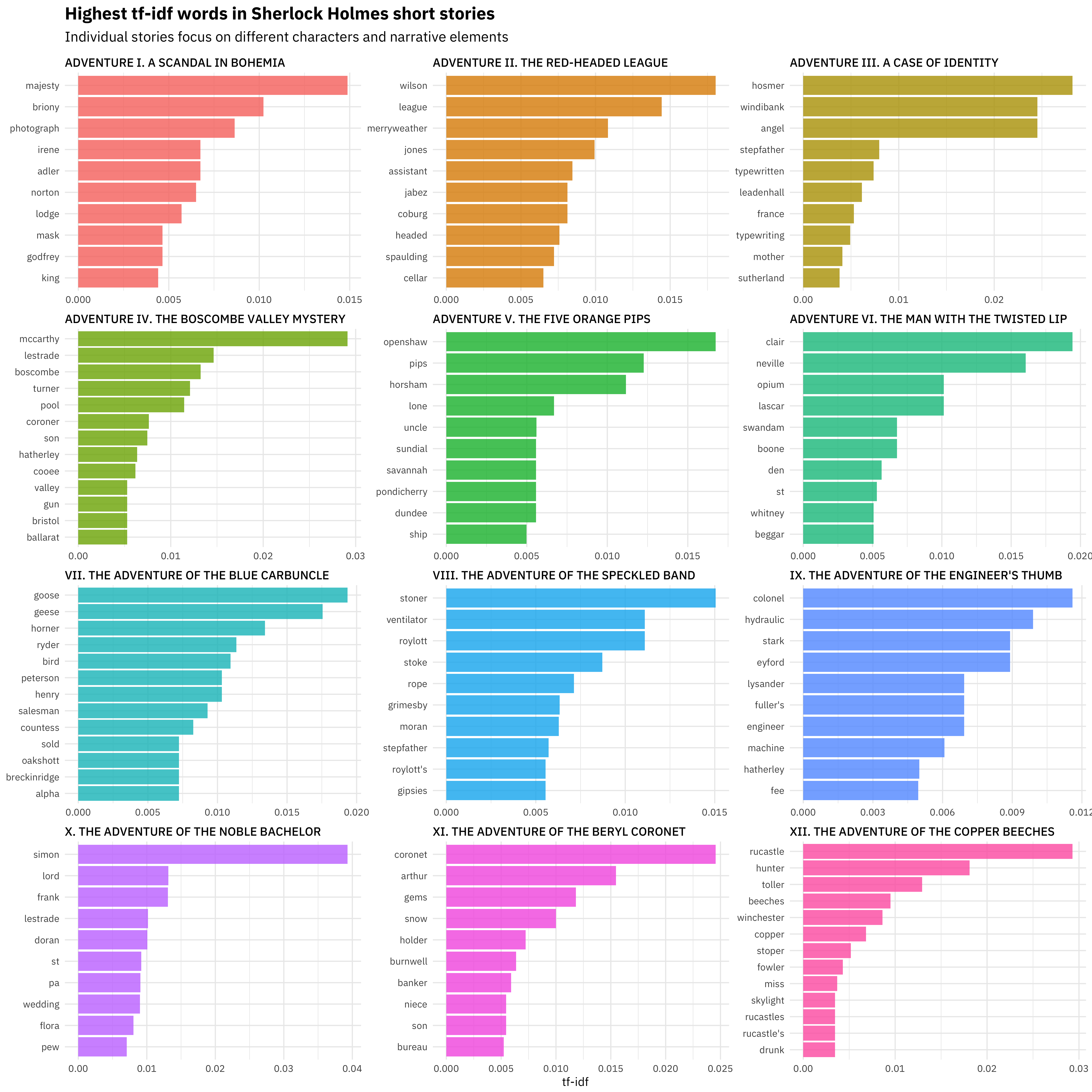
We see lots of proper names here, as well as specific narrative elements for individual stories, like GEESE. 🐦 Exploring tf-idf can be helpful before training topic models.
Speaking of which… let’s get started on a topic model! I am really a fan of the stm package these days because it is easy to install (no rJava dependency! 💀), it is fast (written in Rcpp! 😎), and I have gotten excellent results when experimenting with it. The stm() function take as its input a document-term matrix, either as a sparse matrix or a dfm from quanteda.
library(quanteda)
library(stm)

sherlock_dfm <- tidy_sherlock %>%
    count(story, word, sort = TRUE) %>%
    cast_dfm(story, word, n)

sherlock_sparse <- tidy_sherlock %>%
    count(story, word, sort = TRUE) %>%
    cast_sparse(story, word, n)
You could use either of these objects (sherlock_dfm or sherlock_sparse) as the input to stm(); in the video, I use the quanteda object, so let’s go with that. In this example I am training a topic model with 6 topics, but the stm includes lots of functions and support for choosing an appropriate number of topics for your model.
topic_model <- stm(sherlock_dfm, K = 6,
                   verbose = FALSE, init.type = "Spectral")
The stm package has a summary() method for trained topic models like these that will print out some details to your screen, but I want to get back to a tidy data frame so I can use dplyr and ggplot2 for data manipulation and data visualization. I can use tidy() on the output of an stm model, and then I will get the probabilities that each word is generated from each topic.
td_beta <- tidy(topic_model)

td_beta %>%
    group_by(topic) %>%
    top_n(10, beta) %>%
    ungroup() %>%
    mutate(topic = paste0("Topic ", topic),
           term = reorder_within(term, beta, topic)) %>%
    ggplot(aes(term, beta, fill = as.factor(topic))) +
    geom_col(alpha = 0.8, show.legend = FALSE) +
    facet_wrap(~ topic, scales = "free_y") +
    coord_flip() +
    scale_x_reordered() +
    labs(x = NULL, y = expression(beta),
         title = "Highest word probabilities for each topic",
         subtitle = "Different words are associated with different topics")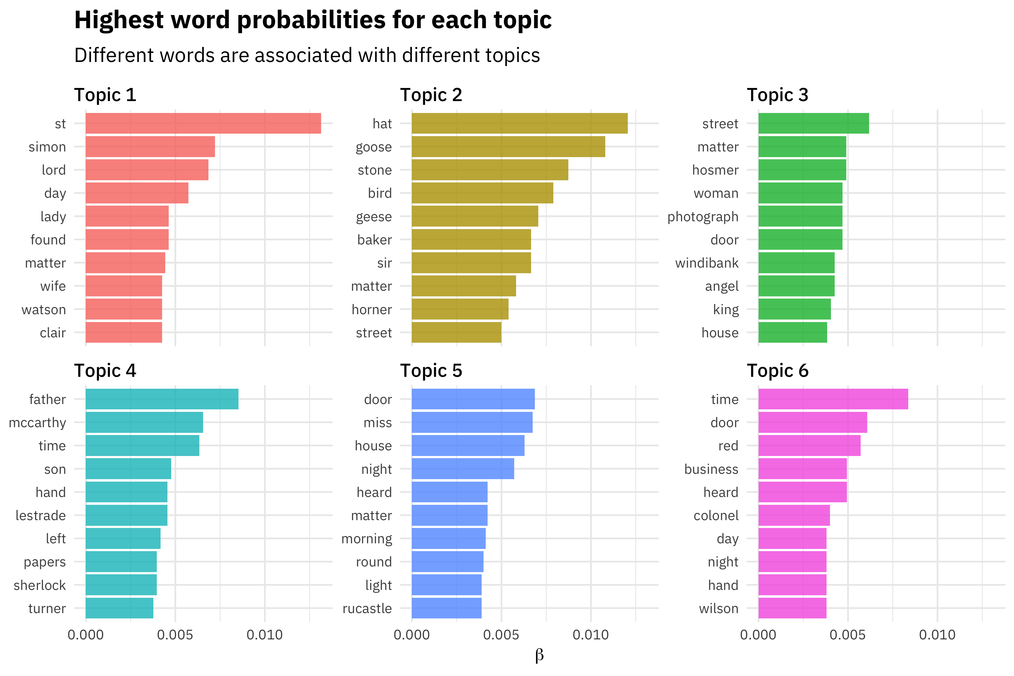
This topic modeling process is a great example of the kind of workflow I often use with text and tidy data principles.
- I use tidy tools like dplyr, tidyr, and ggplot2 for initial data exploration and preparation.
- Then I cast to a non-tidy structure to perform some machine learning algorithm.
- I then tidy the results of my statistical modeling so I can use tidy data principles again to understand my model results.
Now let’s look at another kind of probability we get as output from topic modeling, the probability that each document is generated from each topic.
td_gamma <- tidy(topic_model, matrix = "gamma",
                 document_names = rownames(sherlock_dfm))

ggplot(td_gamma, aes(gamma, fill = as.factor(topic))) +
  geom_histogram(alpha = 0.8, show.legend = FALSE) +
  facet_wrap(~ topic, ncol = 3) +
  labs(title = "Distribution of document probabilities for each topic",
       subtitle = "Each topic is associated with 1-3 stories",
       y = "Number of stories", x = expression(gamma))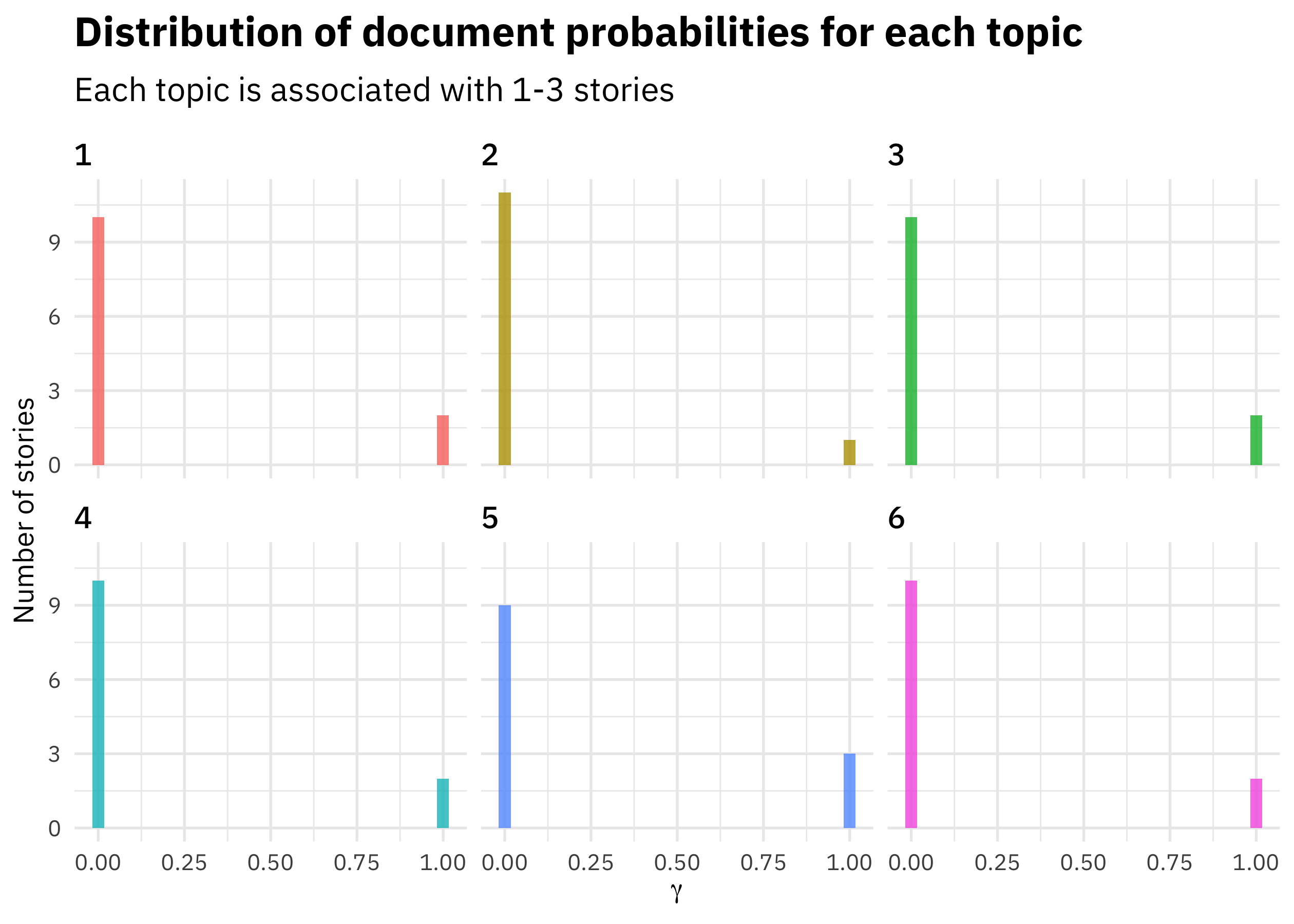
In this case, each short story is strongly associated with a single topic. Topic modeling doesn’t always work out this way, but I built a model here with a small number of documents (only 12) and a relatively large number of topics compared to the number of documents. In any case, this is how we interpret these gamma probabilities; they tell us which topics are coming from which documents.
I built a Shiny app to explore the results of this topic modeling procedure in more detail.
We can see some interesting things; there are shifts through the collection as topic 3 stories come at the beginning and topic 5 stories come at the end. Topic 5 focuses on words that sound like spooky mysteries happening at night, in houses with doors, and events that you see or hear, topic 1 is about lords, ladies, and wives, and topic 2 is about… GEESE. You can use each tab in the app to explore the topic modeling results in different ways.
Let me know if you have any questions about using the stm package in this way, or getting started with topic modeling using tidy data principles! Structural topic models allow you to train more complex models as well, with document-level covariates, and the package contains functions to evaluate the performance of your model. I’ve had great results with this package and I am looking forward to putting together more posts about how to use it!