Bootstrap confidence intervals for #TidyTuesday Super Bowl commercials
By Julia Silge in rstats tidymodels
March 4, 2021
This is the latest in my series of
screencasts demonstrating how to use the
tidymodels packages, from starting out with first modeling steps to tuning more complex models. Today’s screencast uses a relatively new function from rsample for quickly finding bootstrap confidence intervals, with this week’s
#TidyTuesday dataset on Super Bowl commercials. 🏈
Here is the code I used in the video, for those who prefer reading instead of or in addition to video.
Explore the data
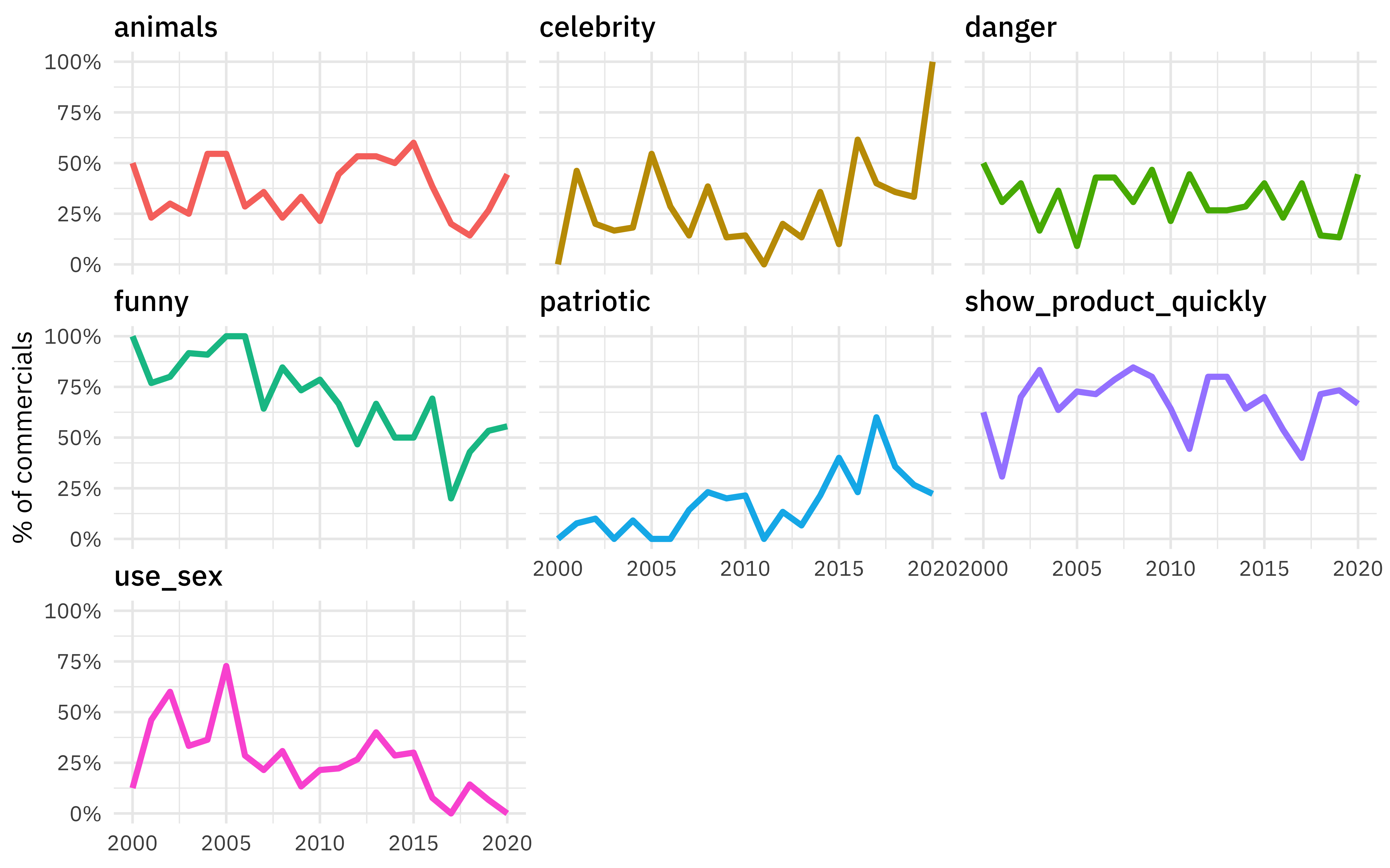
Our modeling goal is to estimate how the characteristics of Super Bowl commercials have changed over time. There aren’t a lot of observations in this data set, and this is an approach that can be used for robust estimates in such situations. Let’s start by reading in the data.
library(tidyverse)
youtube <- read_csv("https://raw.githubusercontent.com/rfordatascience/tidytuesday/master/data/2021/2021-03-02/youtube.csv")
Let’s make one exploratory plot to see how the characteristics of the commercials change over time.
youtube %>%
  select(year, funny:use_sex) %>%
  pivot_longer(funny:use_sex) %>%
  group_by(year, name) %>%
  summarise(prop = mean(value)) %>%
  ungroup() %>%
  ggplot(aes(year, prop, color = name)) +
  geom_line(size = 1.2, show.legend = FALSE) +
  facet_wrap(vars(name)) +
  scale_y_continuous(labels = scales::percent) +
  labs(x = NULL, y = "% of commercials")
Fit a simple model
Although those relationships don’t look perfectly linear, we can use a linear model to estimate if and how much these characteristics are changing with time.
simple_mod <- lm(year ~ funny + show_product_quickly +
  patriotic + celebrity + danger + animals + use_sex,
data = youtube
)

summary(simple_mod)
##
## Call:
## lm(formula = year ~ funny + show_product_quickly + patriotic +
##     celebrity + danger + animals + use_sex, data = youtube)
##
## Residuals:
##      Min       1Q   Median       3Q      Max
## -12.5254  -4.1023   0.1456   3.9662  10.1727
##
## Coefficients:
##                           Estimate Std. Error  t value Pr(>|t|)
## (Intercept)              2011.0838     0.9312 2159.748  < 2e-16 ***
## funnyTRUE                  -2.8979     0.8593   -3.372  0.00087 ***
## show_product_quicklyTRUE    0.7706     0.7443    1.035  0.30160
## patrioticTRUE               2.0455     1.0140    2.017  0.04480 *
## celebrityTRUE               2.4416     0.7767    3.144  0.00188 **
## dangerTRUE                  0.4814     0.7846    0.614  0.54007
## animalsTRUE                 0.1082     0.7330    0.148  0.88274
## use_sexTRUE                -2.4041     0.8175   -2.941  0.00359 **
## ---
## Signif. codes:  0 '***' 0.001 '**' 0.01 '*' 0.05 '.' 0.1 ' ' 1
##
## Residual standard error: 5.391 on 239 degrees of freedom
## Multiple R-squared:  0.178,	Adjusted R-squared:  0.1539
## F-statistic: 7.393 on 7 and 239 DF,  p-value: 4.824e-08
We get statistical properties from this linear model, but we can use bootstrap resampling to get an estimate of the variance in our quantities. In tidymodels, the rsample package has functions to create resamples such as bootstraps.
library(rsample)
bootstraps(youtube, times = 1e3)
## # Bootstrap sampling
## # A tibble: 1,000 x 2
##    splits            id
##    <list>            <chr>
##  1 <split [247/91]>  Bootstrap0001
##  2 <split [247/100]> Bootstrap0002
##  3 <split [247/93]>  Bootstrap0003
##  4 <split [247/87]>  Bootstrap0004
##  5 <split [247/86]>  Bootstrap0005
##  6 <split [247/94]>  Bootstrap0006
##  7 <split [247/98]>  Bootstrap0007
##  8 <split [247/96]>  Bootstrap0008
##  9 <split [247/92]>  Bootstrap0009
## 10 <split [247/89]>  Bootstrap0010
## # … with 990 more rows
This has allowed you to carry out
flexible bootstrapping or permutation steps. However, that’s a lot of steps to get to confidence intervals, especially if you are using a really simple model! In a recent release of rsample, we added a new function reg_intervals() that finds confidence intervals for models like lm() and glm() (as well as models from the
survival package).
set.seed(123)
youtube_intervals <- reg_intervals(year ~ funny + show_product_quickly +
  patriotic + celebrity + danger + animals + use_sex,
data = youtube,
type = "percentile",
keep_reps = TRUE
)

youtube_intervals
## # A tibble: 7 x 7
##   term                   .lower .estimate .upper .alpha .method      .replicates
##   <chr>                   <dbl>     <dbl>  <dbl>  <dbl> <chr>      <list<tibble>
## 1 animalsTRUE            -1.22      0.144  1.51    0.05 percentile   [2,001 × 2]
## 2 celebrityTRUE           0.828     2.46   4.06    0.05 percentile   [2,001 × 2]
## 3 dangerTRUE             -1.01      0.515  2.09    0.05 percentile   [2,001 × 2]
## 4 funnyTRUE              -4.58     -2.91  -1.26    0.05 percentile   [2,001 × 2]
## 5 patrioticTRUE           0.112     2.05   3.88    0.05 percentile   [2,001 × 2]
## 6 show_product_quicklyT… -0.839     0.740  2.23    0.05 percentile   [2,001 × 2]
## 7 use_sexTRUE            -4.04     -2.43  -0.952   0.05 percentile   [2,001 × 2]
All done!
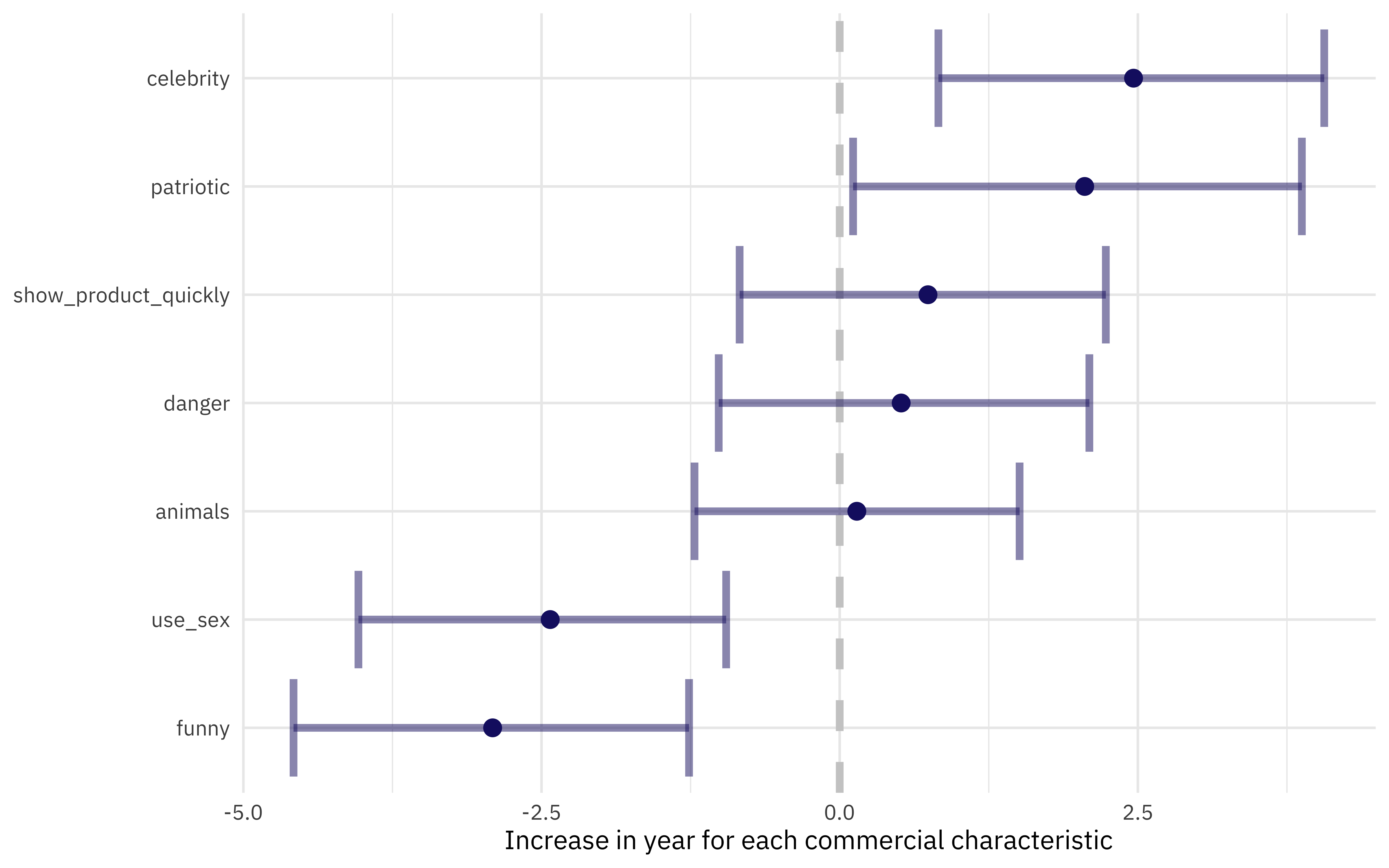
Explore bootstrap results
We can use visualization to explore these results. If we had not set keep_reps = TRUE, we would only have the intervals themselves and could a plot such as this one.
youtube_intervals %>%
  mutate(
    term = str_remove(term, "TRUE"),
    term = fct_reorder(term, .estimate)
  ) %>%
  ggplot(aes(.estimate, term)) +
  geom_vline(xintercept = 0, size = 1.5, lty = 2, color = "gray80") +
  geom_errorbarh(aes(xmin = .lower, xmax = .upper),
    size = 1.5, alpha = 0.5, color = "midnightblue"
  ) +
  geom_point(size = 3, color = "midnightblue") +
  labs(
    x = "Increase in year for each commercial characteristic",
    y = NULL
  )
Since we did keep the individual replicates, we can look at the distributions.
youtube_intervals %>%
  mutate(
    term = str_remove(term, "TRUE"),
    term = fct_reorder(term, .estimate)
  ) %>%
  unnest(.replicates) %>%
  ggplot(aes(estimate, fill = term)) +
  geom_vline(xintercept = 0, size = 1.5, lty = 2, color = "gray50") +
  geom_histogram(alpha = 0.8, show.legend = FALSE) +
  facet_wrap(vars(term))
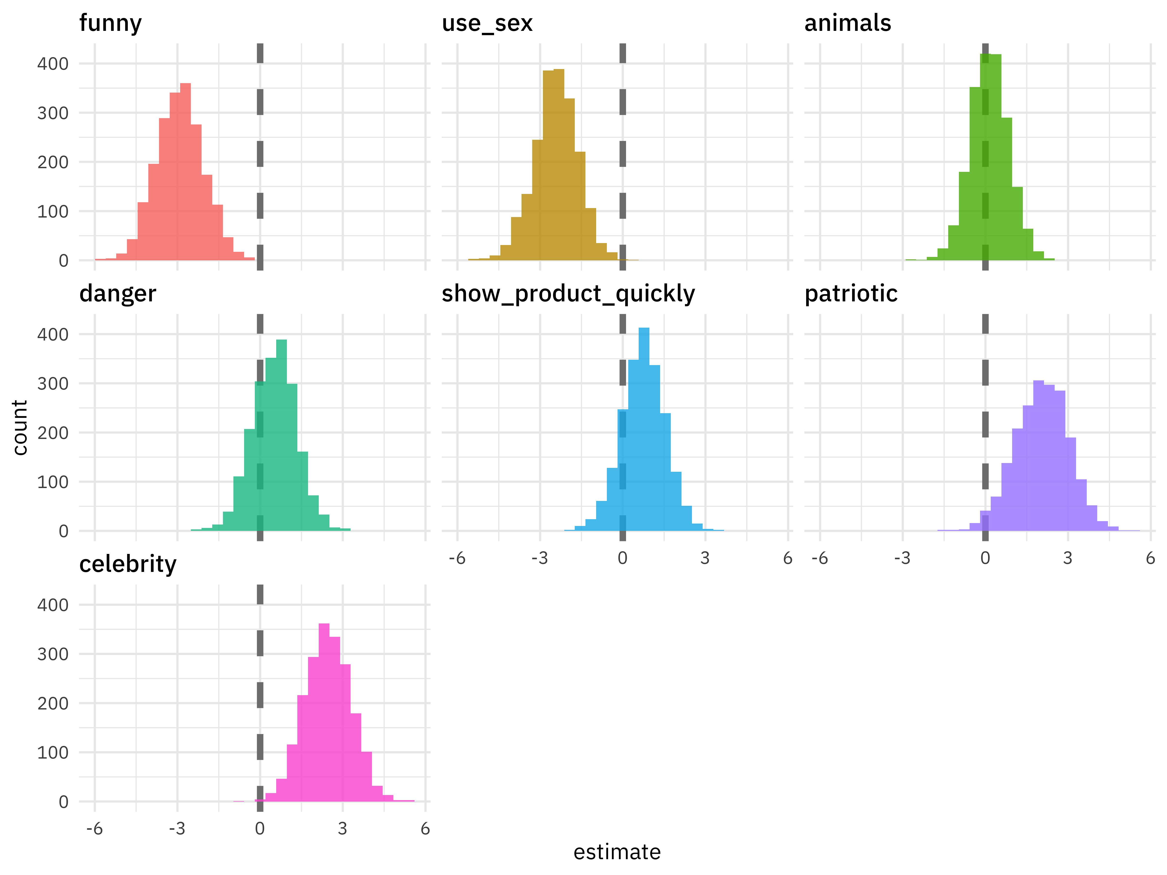
We have evidence that Super Bowl commericals (at least the ones including in this FiveThirtyEight sample) are including less humor and sexual content and more celebrities and patriotic themes.
- Posted on:
- March 4, 2021
- Length:
- 5 minute read, 882 words
- Categories:
- rstats tidymodels
- Tags:
- rstats tidymodels