Word associations from the Small World of Words
By Julia Silge
December 16, 2018
Do you subscribe to the Data is Plural newsletter from Jeremy Singer-Vine? You probably should, because it is a treasure trove of interesting datasets arriving in your email inbox. In the November 28 edition, Jeremy linked to the Small World of Words project, and I was entranced. I love stuff like that, all about words and how people think of them. I have been mulling around a blog post ever since, and today I finally have my post done, so let’s see what’s up!
It’s a Small World
The Small World of Words project focuses on word associations. You can try it out for yourself to see how it works, but the general idea is that the participant is presented with a word (from “telephone” to “journalist” to “yoga”) and is then asked to give their immediate association with that word. The project has collected more than 15 million responses to date, and is still collecting data. You can check out some pre-built visualizations the researchers have put together to explore the dataset, or you can download the data for yourself.
library(tidyverse)

swow_raw <- read_csv("SWOW-EN.R100.csv") %>%
    select(-education, -X1) %>%
    mutate(gender = case_when(gender == "Fe" ~ "Women",
                              gender == "Ma" ~ "Men",
                              gender == "X" ~ "Non-binary"),
           gender = fct_infreq(gender))

swow_raw
## # A tibble: 1,228,200 x 11
## id participantID age gender nativeLanguage country created_at cue R1 R2
## <dbl> <dbl> <dbl> <fct> <chr> <chr> <dttm> <chr> <chr> <chr>
## 1 29 3 33 Women United States Australia 2011-08-12 02:19:38 although nevertheless yet
## 2 30 3 33 Women United States Australia 2011-08-12 02:19:38 deal no cards
## 3 31 3 33 Women United States Australia 2011-08-12 02:19:38 music notes band
## 4 32 3 33 Women United States Australia 2011-08-12 02:19:38 inform tell rat on
## 5 33 3 33 Women United States Australia 2011-08-12 02:19:38 way path via
## 6 34 3 33 Women United States Australia 2011-08-12 02:19:38 none zilch nada
## 7 35 3 33 Women United States Australia 2011-08-12 02:19:38 extra plus special
## 8 36 3 33 Women United States Australia 2011-08-12 02:19:38 will free future
## 9 37 3 33 Women United States Australia 2011-08-12 02:19:38 paper book news
## 10 38 3 33 Women United States Australia 2011-08-12 02:19:38 w v x
## R3
## <chr>
## 1 but
## 2 shake
## 3 rhythm
## 4 <NA>
## 5 method
## 6 zero
## 7 additional
## 8 death
## 9 writing
## 10 what
## # ... with 1,228,190 more rowsThe available dataset as it exists when I downloaded it includes 1,228,200 word associations (each of which involve four words, i.e. three connections) by 83,864 unique participants. When a participant starts on a word association, this project has them move forward through three hops in a chain, from cue to R1 to R2 to R3, and then start over with a new cue. Participants can go through many cues in any given session.
Participants can also report other information about themselves. For example, what is the age distribution?
median_age <- swow_raw %>%
    distinct(participantID, age) %>%
    pull(age) %>%
    median()

swow_raw %>%
    distinct(participantID, age) %>%
    ggplot(aes(age)) +
    geom_histogram(alpha = 0.8, binwidth = 5, fill = "midnightblue") +
    labs(title = "Age distribution of Small World of Words participants",
         subtitle = paste("The median age is", median_age))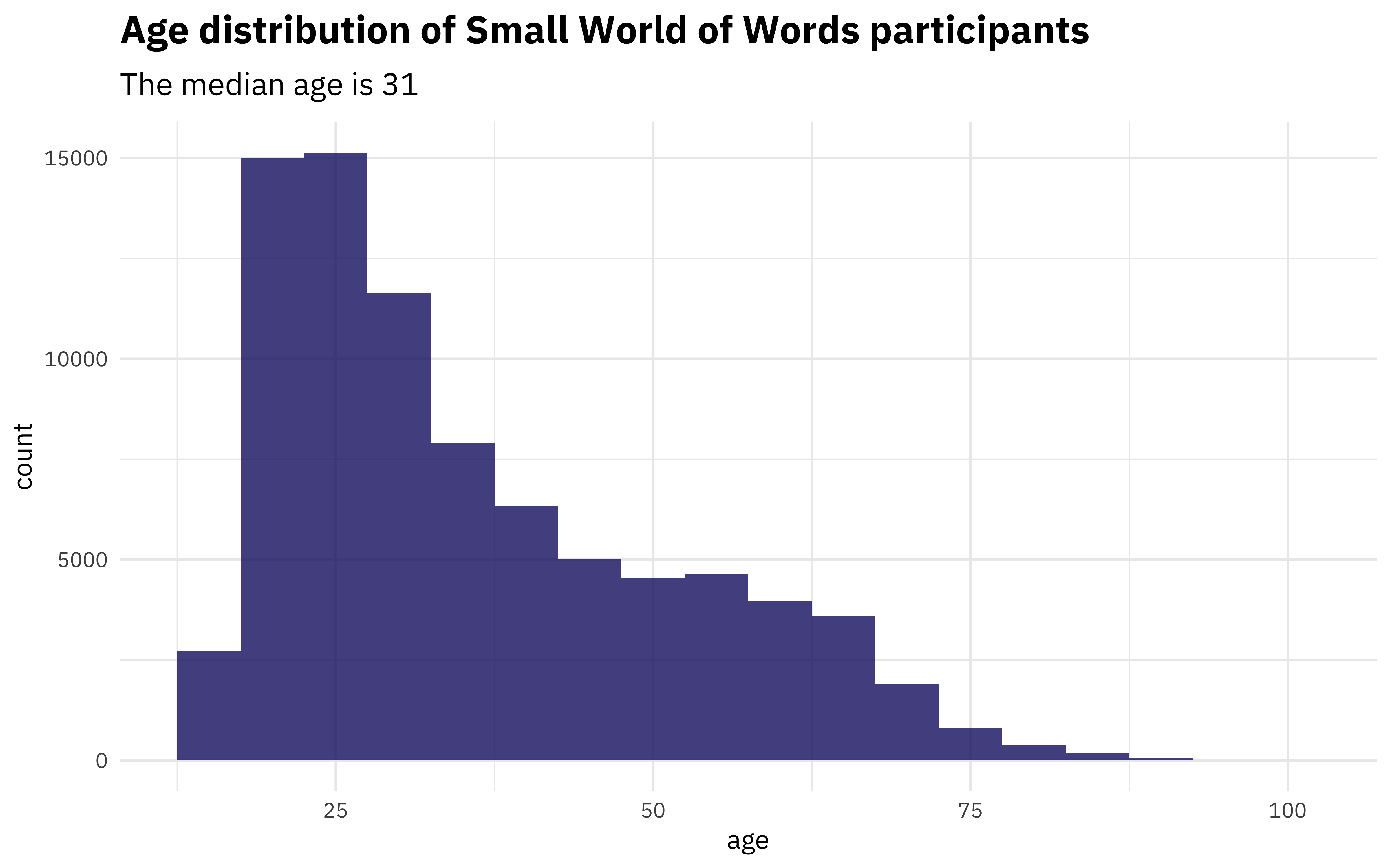
There are lots of young folks represented in this project, as is typical for online surveys. What about gender?
swow_raw %>%
    distinct(participantID, gender) %>%
    count(gender) %>%
    mutate(Percent = n / sum(n)) %>%
    ggplot(aes(fct_reorder(gender, n), Percent)) +
    geom_col(alpha = 0.8, fill = "midnightblue") +
    coord_flip() +
    scale_y_continuous(labels = percent_format(),
                       expand = c(0,0)) +
    labs(x = NULL, y = "% of participants",
         title = "Gender distribution of Small World of Words participants",
         subtitle = "More than 60% of participants identify as women")
In this project, women were more likely to participate than other genders.
This project is international, pulling participants from many native languages. It also allows folks to specify whether they are a US English speaker, a UK English speaker, etc.
native_languages <- swow_raw %>%
    distinct(participantID, nativeLanguage) %>%
    pull(nativeLanguage)

swow_raw %>%
    distinct(participantID, nativeLanguage) %>%
    count(nativeLanguage) %>%
    top_n(15) %>%
    ggplot(aes(fct_reorder(nativeLanguage, n), n)) +
    geom_col(alpha = 0.8, fill = "midnightblue") +
    coord_flip() +
    scale_y_continuous(labels = comma_format(),
                       expand = c(0,0)) +
    labs(x = NULL, y = "Number of participants",
         title = "Native languages of Small World of Words participants",
         subtitle = paste("About", percent(mean(native_languages == "United States")),
                          "of participants say their native language is US English"))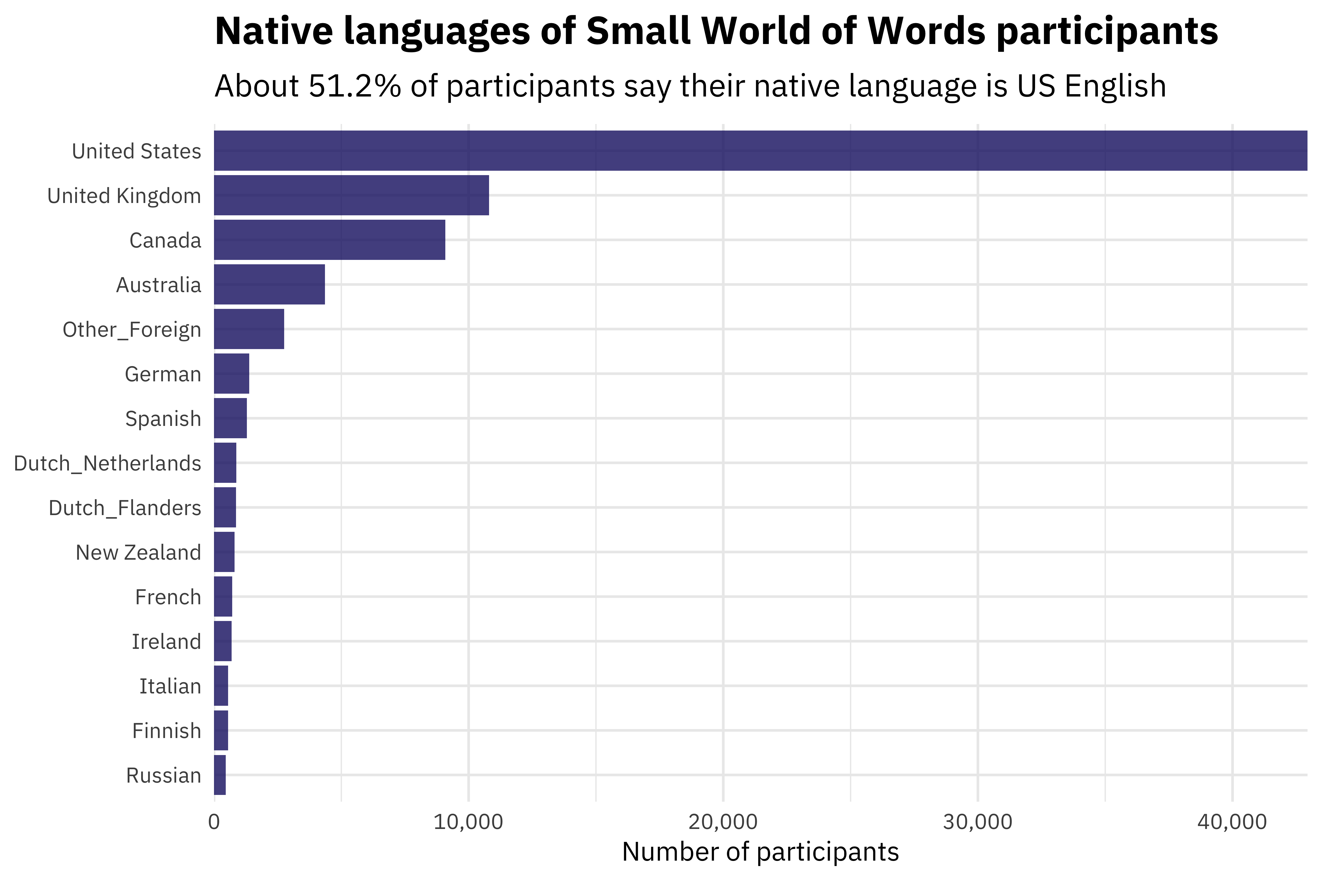
So that’s a little bit of EDA to understand this project and its participants. Now let’s dig into the word associations!
Building forward associations
This is a rich, detailed dataset and there are so many directions we could go with it. In taking a first stab, let’s look at all the forward associations in the whole project. This means we will treat the “hop” from the cue to the first association the same as the “hop” from the first to second association, which certainly isn’t entirely correct. It’s a choice to start from, though.
swow_forward <- swow_raw %>%
    select(from = cue, to = R1, gender, age, nativeLanguage) %>%
    bind_rows(
        swow_raw %>%
            select(from = R1, to = R2, gender, age, nativeLanguage)
    ) %>%
    bind_rows(
        swow_raw %>%
            select(from = R2, to = R3, gender, age, nativeLanguage)
    ) %>%
    filter(!is.na(to))

swow_forward
## # A tibble: 3,403,790 x 5
## from to gender age nativeLanguage
## <chr> <chr> <fct> <dbl> <chr>
## 1 although nevertheless Women 33 United States
## 2 deal no Women 33 United States
## 3 music notes Women 33 United States
## 4 inform tell Women 33 United States
## 5 way path Women 33 United States
## 6 none zilch Women 33 United States
## 7 extra plus Women 33 United States
## 8 will free Women 33 United States
## 9 paper book Women 33 United States
## 10 w v Women 33 United States
## # ... with 3,403,780 more rowsNow that we have all the forward associations, we can find the most common associations for any individual word with some simple dplyr operations. What about… coffee? ☕
swow_forward %>%
    filter(from == "coffee") %>%
    count(to, sort = TRUE)
## # A tibble: 711 x 2
## to n
## <chr> <int>
## 1 tea 80
## 2 milk 33
## 3 drink 31
## 4 Starbucks 28
## 5 caffeine 15
## 6 cup 15
## 7 morning 15
## 8 hot 13
## 9 chocolate 12
## 10 island 12
## # ... with 701 more rowsOr… maybe you are in a holiday Christmas celebratory mood, and want to know what people associate with the word “Christmas”.
swow_forward %>%
    filter(from == "Christmas") %>%
    count(to, sort = TRUE)
## # A tibble: 759 x 2
## to n
## <chr> <int>
## 1 birthday 56
## 2 holiday 45
## 3 tree 43
## 4 Santa 34
## 5 snow 33
## 6 happy 31
## 7 red 29
## 8 presents 28
## 9 winter 24
## 10 Jesus 19
## # ... with 749 more rowsComparing groups
This project recorded information about the participants themselves, so we can dig into how different kinds of people associate words. For example, let’s start with gender and comparing folks who identify as men and women. What differences do we see with the word “water”?
swow_forward %>%
    filter(from == "water",
           gender %in% c("Men", "Women")) %>%
    group_by(to) %>%
    filter(n() > 30) %>%
    ungroup %>%
    count(gender, to, sort = TRUE) %>%
    spread(gender, n, fill = 0) %>%
    mutate_if(is.numeric, funs((. + 1) / (sum(.) + 1))) %>%
    mutate(logratio = log2(Women / Men)) %>%
    top_n(15, abs(logratio)) %>%
    ggplot(aes(fct_reorder(to, logratio), logratio,
               fill = logratio < 0)) +
    geom_col(alpha = 0.8, show.legend = FALSE) +
    coord_flip() +
    labs(x = NULL, y  = "log odds ratio (Women/Men)",
         title = "What words do Small World of Words' participants associate with water?",
subtitle = "Women are more likely to mention sinks and baths\nMen are more likely to say steam and air") 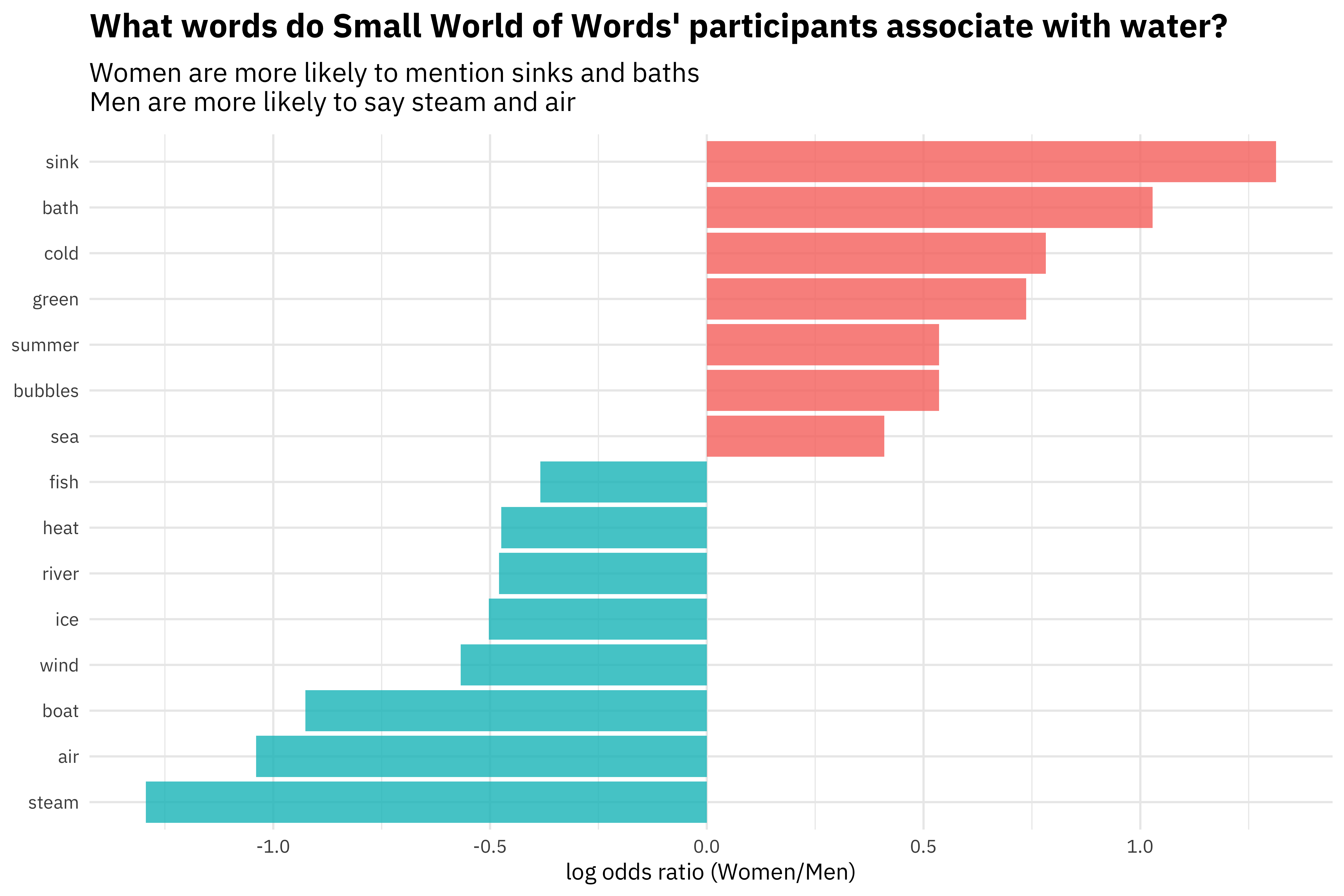
Notice the dramatic contrasts between domestic water uses like sinks and baths with more scientific word about water like steam. We see how socialized and differentiated women’s language is, even with something that seems neutral like water.
What about differences between US and UK English?
swow_forward %>%
    filter(from == "love",
           nativeLanguage %in% c("United States", "United Kingdom")) %>%
    group_by(to) %>%
    filter(n() > 30) %>%
    ungroup %>%
    count(nativeLanguage, to, sort = TRUE) %>%
    spread(nativeLanguage, n, fill = 0) %>%
    mutate_if(is.numeric, funs((. + 1) / (sum(.) + 1))) %>%
    mutate(logratio = log2(`United States` / `United Kingdom`)) %>%
    ggplot(aes(fct_reorder(to, logratio), logratio,
               fill = logratio < 0)) +
    geom_col(alpha = 0.8, show.legend = FALSE) +
    coord_flip() +
    labs(x = NULL, y  = "log odds ratio (US/UK)",
         title = "What words do Small World of Words' participants associate with love?",
subtitle = "US participants associate love with hate\nUK participants feel more affectionate") 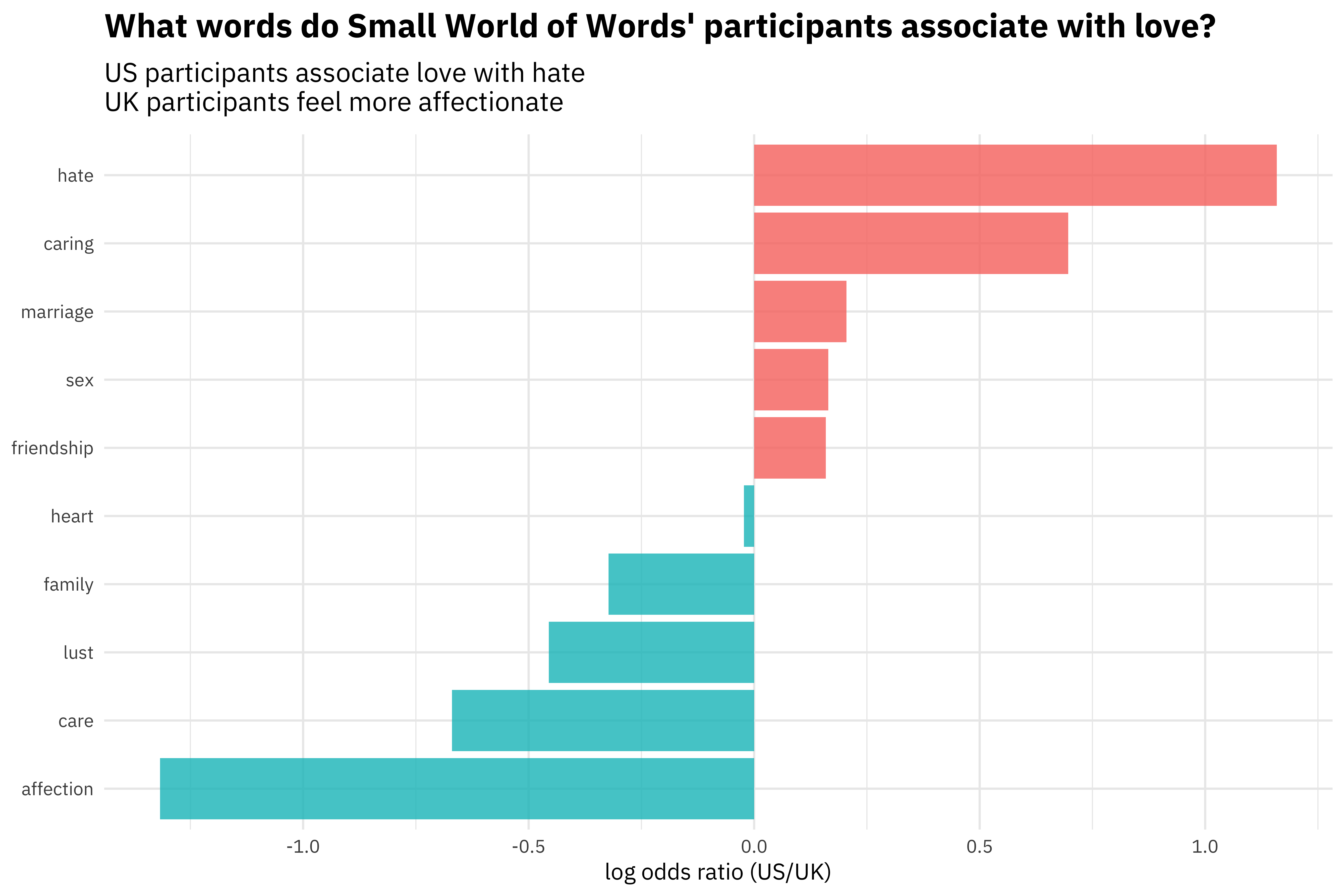
Well, alrighty then. 😳
Changes with age
We can apply some functional programming and modeling to look at how these word associations change with age. Let’s take the word “money”, and start by calculating, for 5-year bins, the number and proportion of words associated for each bin.
swow_freq <- swow_forward %>%
    filter(from == "money",
           age < 80) %>%
    mutate(age = age %/% 5 * 5) %>%
    count(age, to) %>%
    complete(age, to, fill = list(n = 0)) %>%
    group_by(age) %>%
    mutate(age_total = sum(n),
           percent = n / age_total) %>%
    ungroup %>%
    group_by(to) %>%
    filter(sum(n) > 25) %>%
    ungroup

swow_freq
## # A tibble: 741 x 5
## age to n age_total percent
## <dbl> <chr> <dbl> <dbl> <dbl>
## 1 15 bank 47 1118 0.0420
## 2 15 banks 7 1118 0.00626
## 3 15 bills 2 1118 0.00179
## 4 15 business 11 1118 0.00984
## 5 15 buy 7 1118 0.00626
## 6 15 car 4 1118 0.00358
## 7 15 cash 30 1118 0.0268
## 8 15 change 5 1118 0.00447
## 9 15 charity 5 1118 0.00447
## 10 15 cheap 5 1118 0.00447
## # ... with 731 more rowsNow let’s fit some models using glm() since this is count data to predict the counts out of the total for each age bin from the age. We can then tidy() the output of the modeling, adjust the p-values for multiple comparisons since we looked at a bunch of words at one time, and make a volcano-style plot to compare the effect size with the p-value.
library(broom)
library(ggrepel)

slopes <- swow_freq %>%
    nest(-to) %>%
    mutate(models = map(data, ~ glm(cbind(n, age_total) ~ age, .,
                                    family = "binomial"))) %>%
    unnest(map(models, tidy)) %>%
    filter(term == "age") %>%
    arrange(estimate) %>%
    mutate(p.value = p.adjust(p.value))

slopes %>%
    ggplot(aes(estimate, p.value)) +
    geom_vline(xintercept = 0, lty = 2, alpha = 0.7, color = "gray50") +
    geom_point(color = "midnightblue", alpha = 0.8, size = 2.5) +
    scale_y_log10() +
    geom_text(data = filter(slopes,
                            p.value >= 0.5),
              aes(label = to),
              family = "IBMPlexSans",
              vjust = 0, nudge_y = 0.02,
              check_overlap = TRUE) +
    geom_text_repel(data = filter(slopes,
                                  p.value < 0.5),
                    aes(label = to),
                    family = "IBMPlexSans") +
    labs(x = "Estimated change with age",
         y = "Adjusted p-value",
         title = "What words do Small World of Words' participants associate with money?",
         subtitle = "Older participants are more likely to say stocks or dollars\nYounger participants are more likely to talk about a job or the color green")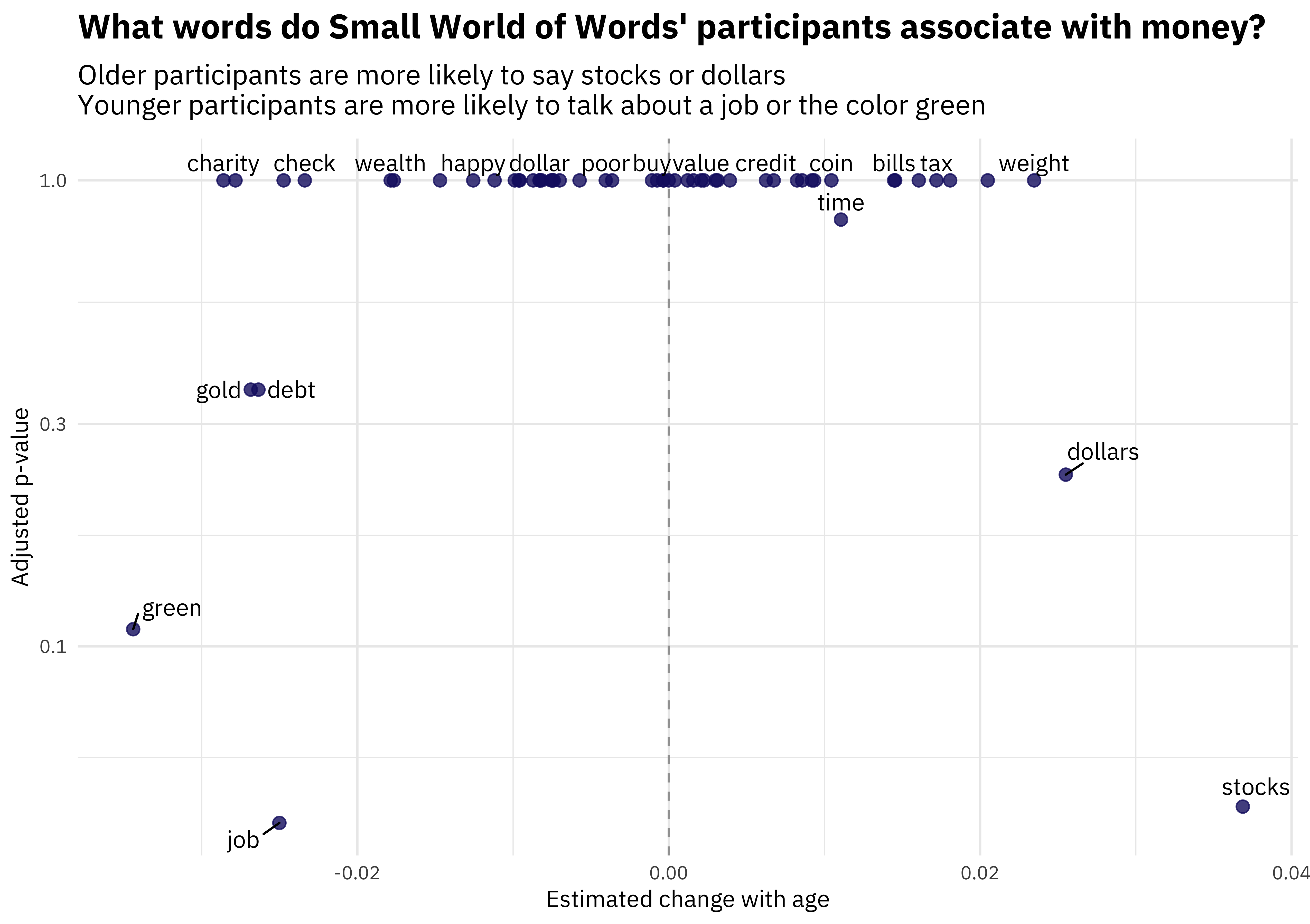
The younger someone is, the more likely they are to associate money with a job, or the color green or gold. The older someone is, the more likely they are to associate money with dollars and stocks. Let’s look at the top terms associated with money that exhibit change with age in terms of a small p-value.
slopes %>%
    top_n(6, -p.value) %>%
    inner_join(swow_freq) %>%
    ggplot(aes(age, percent)) +
    geom_point() +
    geom_smooth() +
    facet_wrap(~ to) +
    scale_y_continuous(labels = percent_format()) +
    labs(x = "Age of participant",
         y = "Frequency of word in association with money",
         title = "What words do Small World of Words' participants associate with money?",
         subtitle = "Words like debt and gold decrease in frequency with age")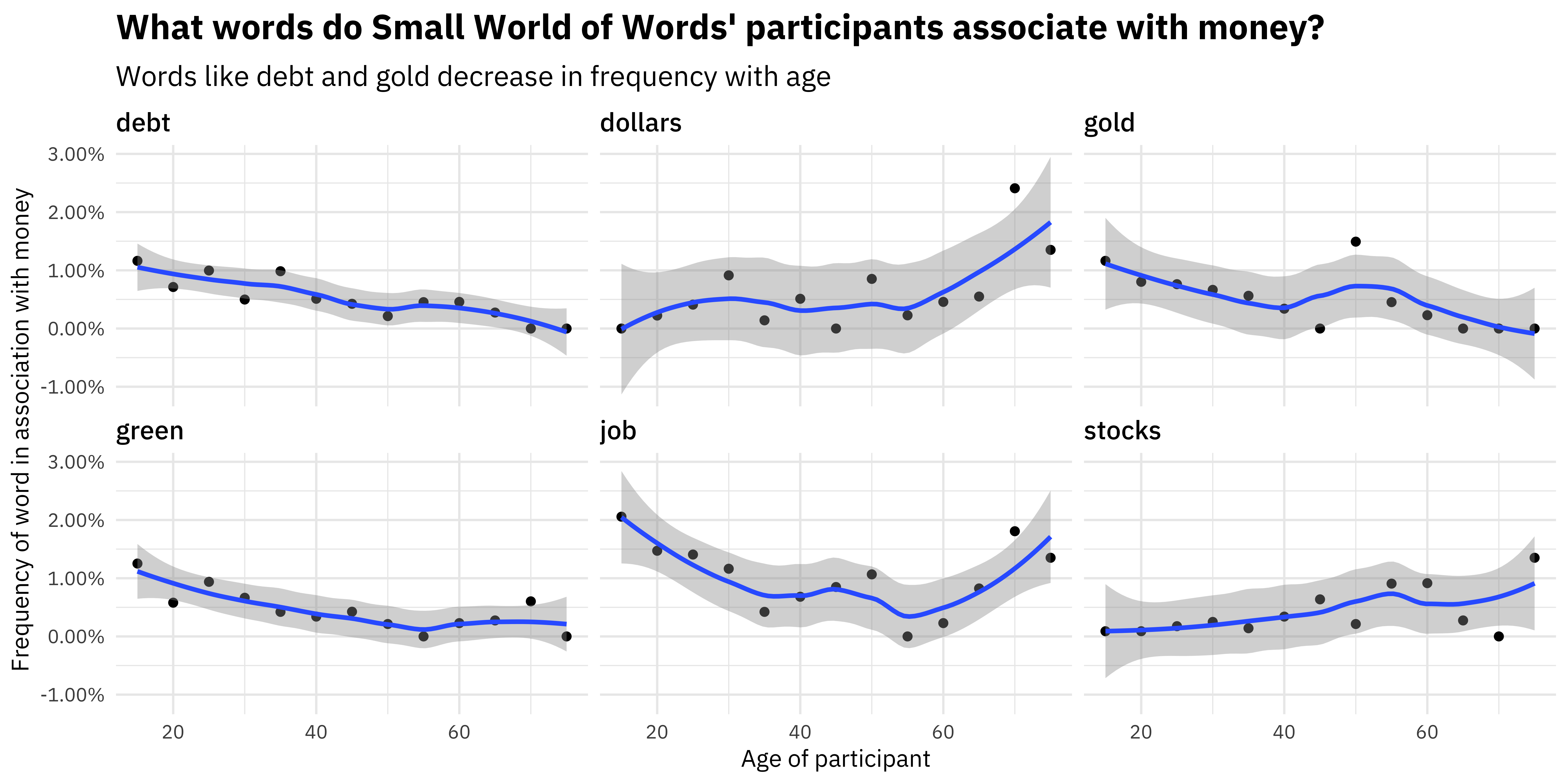
Younger respondents were more likely to associate words like DEBT with money. 😵
The End
There is so much more that could be done with this dataset. You could build a network data structure between the words and do various kinds of network analysis, and I didn’t touch any of the differences in the intial cue vs. the later hops. Notice that this dataset is all about words, but I didn’t ever load the tidytext package for this analysis. The researchers who built this dataset have already done much of the hard work of processing this data, and it is more like structured data that happens to be about language, rather than unstructured text data. Let me know if you have any questions!