Tune XGBoost with tidymodels and #TidyTuesday beach volleyball
in rstats tidymodels
May 21, 2020
Lately I’ve been publishing
screencasts demonstrating how to use the
tidymodels framework, starting from just getting started. Today’s screencast explores a more advanced topic in how to tune an XGBoost classification model using with this week’s
#TidyTuesday dataset on beach volleyball. 🏐
Here is the code I used in the video, for those who prefer reading instead of or in addition to video.
Explore the data
Our modeling goal is to predict whether a beach volleyball team of two won their match based on game play stats like errors, blocks, attacks, etc from this week’s #TidyTuesday dataset . This dataset is quite extensive so it’s a great opportunity to try a more powerful machine learning algorithm like XGBoost. This model has lots of tuning parameters!
vb_matches <- readr::read_csv('https://raw.githubusercontent.com/rfordatascience/tidytuesday/master/data/2020/2020-05-19/vb_matches.csv', guess_max = 76000)

vb_matches
## # A tibble: 76,756 x 65
##    circuit tournament country  year date       gender match_num w_player1
##    <chr>   <chr>      <chr>   <dbl> <date>     <chr>      <dbl> <chr>
##  1 AVP     Huntingto… United…  2002 2002-05-24 M              1 Kevin Wo…
##  2 AVP     Huntingto… United…  2002 2002-05-24 M              2 Brad Tor…
##  3 AVP     Huntingto… United…  2002 2002-05-24 M              3 Eduardo …
##  4 AVP     Huntingto… United…  2002 2002-05-24 M              4 Brent Do…
##  5 AVP     Huntingto… United…  2002 2002-05-24 M              5 Albert H…
##  6 AVP     Huntingto… United…  2002 2002-05-24 M              6 Jason Ri…
##  7 AVP     Huntingto… United…  2002 2002-05-24 M              7 Aaron Bo…
##  8 AVP     Huntingto… United…  2002 2002-05-24 M              8 Canyon C…
##  9 AVP     Huntingto… United…  2002 2002-05-24 M              9 Dax Hold…
## 10 AVP     Huntingto… United…  2002 2002-05-24 M             10 Mark Wil…
## # … with 76,746 more rows, and 57 more variables: w_p1_birthdate <date>,
## #   w_p1_age <dbl>, w_p1_hgt <dbl>, w_p1_country <chr>, w_player2 <chr>,
## #   w_p2_birthdate <date>, w_p2_age <dbl>, w_p2_hgt <dbl>, w_p2_country <chr>,
## #   w_rank <chr>, l_player1 <chr>, l_p1_birthdate <date>, l_p1_age <dbl>,
## #   l_p1_hgt <dbl>, l_p1_country <chr>, l_player2 <chr>, l_p2_birthdate <date>,
## #   l_p2_age <dbl>, l_p2_hgt <dbl>, l_p2_country <chr>, l_rank <chr>,
## #   score <chr>, duration <time>, bracket <chr>, round <chr>,
## #   w_p1_tot_attacks <dbl>, w_p1_tot_kills <dbl>, w_p1_tot_errors <dbl>,
## #   w_p1_tot_hitpct <dbl>, w_p1_tot_aces <dbl>, w_p1_tot_serve_errors <dbl>,
## #   w_p1_tot_blocks <dbl>, w_p1_tot_digs <dbl>, w_p2_tot_attacks <dbl>,
## #   w_p2_tot_kills <dbl>, w_p2_tot_errors <dbl>, w_p2_tot_hitpct <dbl>,
## #   w_p2_tot_aces <dbl>, w_p2_tot_serve_errors <dbl>, w_p2_tot_blocks <dbl>,
## #   w_p2_tot_digs <dbl>, l_p1_tot_attacks <dbl>, l_p1_tot_kills <dbl>,
## #   l_p1_tot_errors <dbl>, l_p1_tot_hitpct <dbl>, l_p1_tot_aces <dbl>,
## #   l_p1_tot_serve_errors <dbl>, l_p1_tot_blocks <dbl>, l_p1_tot_digs <dbl>,
## #   l_p2_tot_attacks <dbl>, l_p2_tot_kills <dbl>, l_p2_tot_errors <dbl>,
## #   l_p2_tot_hitpct <dbl>, l_p2_tot_aces <dbl>, l_p2_tot_serve_errors <dbl>,
## #   l_p2_tot_blocks <dbl>, l_p2_tot_digs <dbl>
This dataset has the match stats like serve errors, kills, and so forth divided out by the two players for each team, but we want those combined together because we are going to make a prediction per team (i.e. what makes a team more likely to win). Let’s include predictors like gender, circuit, and year in our model along with the per-match statistics. Let’s omit matches with NA values because we don’t have all kinds of statistics measured for all matches.
vb_parsed <- vb_matches %>%
  transmute(
    circuit,
    gender,
    year,
    w_attacks = w_p1_tot_attacks + w_p2_tot_attacks,
    w_kills = w_p1_tot_kills + w_p2_tot_kills,
    w_errors = w_p1_tot_errors + w_p2_tot_errors,
    w_aces = w_p1_tot_aces + w_p2_tot_aces,
    w_serve_errors = w_p1_tot_serve_errors + w_p2_tot_serve_errors,
    w_blocks = w_p1_tot_blocks + w_p2_tot_blocks,
    w_digs = w_p1_tot_digs + w_p2_tot_digs,
    l_attacks = l_p1_tot_attacks + l_p2_tot_attacks,
    l_kills = l_p1_tot_kills + l_p2_tot_kills,
    l_errors = l_p1_tot_errors + l_p2_tot_errors,
    l_aces = l_p1_tot_aces + l_p2_tot_aces,
    l_serve_errors = l_p1_tot_serve_errors + l_p2_tot_serve_errors,
    l_blocks = l_p1_tot_blocks + l_p2_tot_blocks,
    l_digs = l_p1_tot_digs + l_p2_tot_digs
  ) %>%
  na.omit()
Still plenty of data! Next, let’s create separate dataframes for the winners and losers of each match, and then bind them together. I am using functions like rename_with() from the
upcoming dplyr 1.0 release here.
winners <- vb_parsed %>%
  select(circuit, gender, year,
         w_attacks:w_digs) %>%
  rename_with(~ str_remove_all(., "w_"), w_attacks:w_digs) %>%
  mutate(win = "win")

losers <- vb_parsed %>%
  select(circuit, gender, year,
         l_attacks:l_digs) %>%
  rename_with(~ str_remove_all(., "l_"), l_attacks:l_digs) %>%
  mutate(win = "lose")

vb_df <- bind_rows(winners, losers) %>%
  mutate_if(is.character, factor)
This is a similar data prep approach to Joshua Cook.
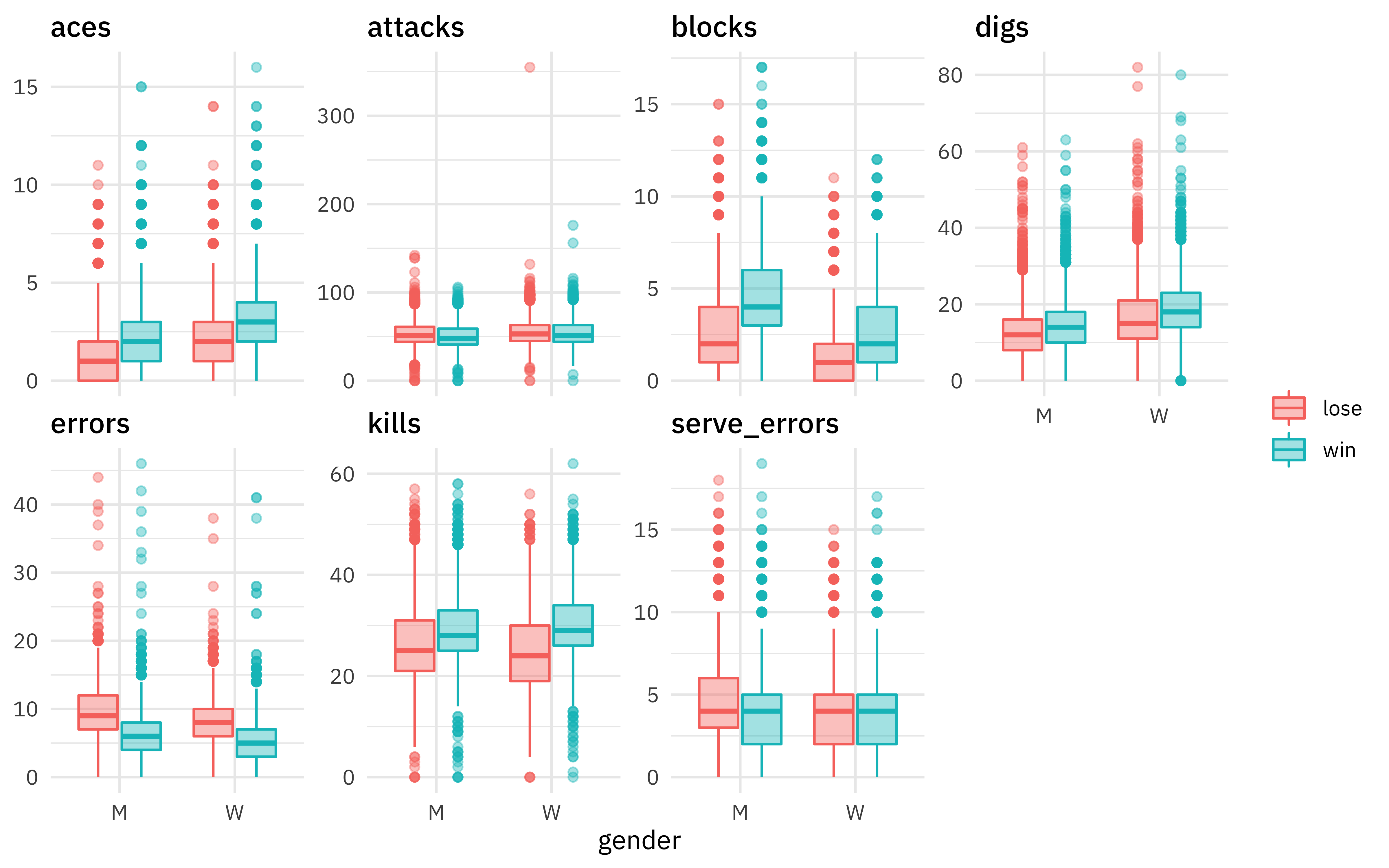
Exploratory data analysis is always important before modeling. Let’s make one plot to explore the relationships in this data.
vb_df %>%
  pivot_longer(attacks:digs, names_to = "stat", values_to = "value") %>%
  ggplot(aes(gender, value, fill = win, color = win)) +
  geom_boxplot(alpha = 0.4) +
  facet_wrap(~stat, scales = "free_y", nrow = 2) +
  labs(y = NULL, color = NULL, fill = NULL)

We can see differences in errors and blocks especially. There are lots more great examples of #TidyTuesday EDA out there to explore on Twitter!
Build a model
We can start by loading the tidymodels metapackage, and splitting our data into training and testing sets.
library(tidymodels)

set.seed(123)
vb_split <- initial_split(vb_df, strata = win)
vb_train <- training(vb_split)
vb_test <- testing(vb_split)
An XGBoost model is based on trees, so we don’t need to do much preprocessing for our data; we don’t need to worry about the factors or centering or scaling our data. Let’s just go straight to setting up our model specification. Sounds great, right? On the other hand, we are going to tune a lot of model hyperparameters.
xgb_spec <- boost_tree(
  trees = 1000,
  tree_depth = tune(), min_n = tune(),
  loss_reduction = tune(),                     ## first three: model complexity
  sample_size = tune(), mtry = tune(),         ## randomness
  learn_rate = tune()                          ## step size
) %>%
  set_engine("xgboost") %>%
  set_mode("classification")

xgb_spec
## Boosted Tree Model Specification (classification)
##
## Main Arguments:
##   mtry = tune()
##   trees = 1000
##   min_n = tune()
##   tree_depth = tune()
##   learn_rate = tune()
##   loss_reduction = tune()
##   sample_size = tune()
##
## Computational engine: xgboost
YIKES. 😩 Well, let’s set up possible values for these hyperparameters to try. Let’s use a space-filling design so we can cover the hyperparameter space as well as possible.
xgb_grid <- grid_latin_hypercube(
  tree_depth(),
  min_n(),
  loss_reduction(),
  sample_size = sample_prop(),
  finalize(mtry(), vb_train),
  learn_rate(),
  size = 30
)

xgb_grid
## # A tibble: 30 x 6
##    tree_depth min_n loss_reduction sample_size  mtry    learn_rate
##         <int> <int>          <dbl>       <dbl> <int>         <dbl>
##  1         13     9    0.000000191       0.488     6 0.000147
##  2          4    17    0.0000121         0.661    10 0.00000000287
##  3          7    18    0.0000432         0.151     2 0.0713
##  4         12    22    0.00000259        0.298     8 0.0000759
##  5         10    35   16.1               0.676     6 0.00000000111
##  6          4    21    0.673             0.957     7 0.00000000786
##  7          7    25    0.244             0.384     9 0.0000000469
##  8          7     3    8.48              0.775     6 0.000000555
##  9          6     8    0.0000915         0.522     6 0.00000106
## 10         11    37    0.00000109        0.886     9 0.0000000136
## # … with 20 more rows
Notice that we had to treat mtry() differently because it depends on the actual number of predictors in the data.
Let’s put the model specification into a workflow for convenience. Since we don’t have any complicated data preprocessing, we can use add_formula() as our data preprocessor.
xgb_wf <- workflow() %>%
  add_formula(win ~ .) %>%
  add_model(xgb_spec)

xgb_wf
## ══ Workflow ═══════════════════════════════════════════════════════════
## Preprocessor: Formula
## Model: boost_tree()
##
## ── Preprocessor ───────────────────────────────────────────────────────
## win ~ .
##
## ── Model ──────────────────────────────────────────────────────────────
## Boosted Tree Model Specification (classification)
##
## Main Arguments:
##   mtry = tune()
##   trees = 1000
##   min_n = tune()
##   tree_depth = tune()
##   learn_rate = tune()
##   loss_reduction = tune()
##   sample_size = tune()
##
## Computational engine: xgboost
Next, let’s create cross-validation resamples for tuning our model.
set.seed(123)
vb_folds <- vfold_cv(vb_train, strata = win)

vb_folds
## #  10-fold cross-validation using stratification
## # A tibble: 10 x 2
##    splits               id
##    <named list>         <chr>
##  1 <split [19.3K/2.1K]> Fold01
##  2 <split [19.3K/2.1K]> Fold02
##  3 <split [19.3K/2.1K]> Fold03
##  4 <split [19.3K/2.1K]> Fold04
##  5 <split [19.3K/2.1K]> Fold05
##  6 <split [19.3K/2.1K]> Fold06
##  7 <split [19.3K/2.1K]> Fold07
##  8 <split [19.3K/2.1K]> Fold08
##  9 <split [19.3K/2.1K]> Fold09
## 10 <split [19.4K/2.1K]> Fold10
IT’S TIME TO TUNE. We use tune_grid() with our tuneable workflow, our resamples, and our grid of parameters to try. Let’s use control_grid(save_pred = TRUE) so we can explore the predictions afterwards.
doParallel::registerDoParallel()

set.seed(234)
xgb_res <- tune_grid(
  xgb_wf,
  resamples = vb_folds,
  grid = xgb_grid,
  control = control_grid(save_pred = TRUE)
)

xgb_res
## #  10-fold cross-validation using stratification
## # A tibble: 10 x 5
##    splits             id     .metrics        .notes         .predictions
##    <named list>       <chr>  <list>          <list>         <list>
##  1 <split [19.3K/2.1… Fold01 <tibble [60 × … <tibble [0 × … <tibble [64,500 × 1…
##  2 <split [19.3K/2.1… Fold02 <tibble [60 × … <tibble [0 × … <tibble [64,500 × 1…
##  3 <split [19.3K/2.1… Fold03 <tibble [60 × … <tibble [0 × … <tibble [64,500 × 1…
##  4 <split [19.3K/2.1… Fold04 <tibble [60 × … <tibble [0 × … <tibble [64,500 × 1…
##  5 <split [19.3K/2.1… Fold05 <tibble [60 × … <tibble [0 × … <tibble [64,500 × 1…
##  6 <split [19.3K/2.1… Fold06 <tibble [60 × … <tibble [0 × … <tibble [64,500 × 1…
##  7 <split [19.3K/2.1… Fold07 <tibble [60 × … <tibble [0 × … <tibble [64,500 × 1…
##  8 <split [19.3K/2.1… Fold08 <tibble [60 × … <tibble [0 × … <tibble [64,500 × 1…
##  9 <split [19.3K/2.1… Fold09 <tibble [60 × … <tibble [0 × … <tibble [64,500 × 1…
## 10 <split [19.4K/2.1… Fold10 <tibble [60 × … <tibble [0 × … <tibble [64,440 × 1…
This takes a while to finish on my computer (and makes my fans run!) but we did it. 💪
Explore results
We can explore the metrics for all these models.
collect_metrics(xgb_res)
## # A tibble: 60 x 11
##     mtry min_n tree_depth learn_rate loss_reduction sample_size .metric
##    <int> <int>      <int>      <dbl>          <dbl>       <dbl> <chr>
##  1     1    23          9    1.64e-3   0.00000854         0.117 accura…
##  2     1    23          9    1.64e-3   0.00000854         0.117 roc_auc
##  3     2    18          7    7.13e-2   0.0000432          0.151 accura…
##  4     2    18          7    7.13e-2   0.0000432          0.151 roc_auc
##  5     2    32          3    1.30e-7   1.16               0.497 accura…
##  6     2    32          3    1.30e-7   1.16               0.497 roc_auc
##  7     2    40         10    3.31e-4   0.0000000486       0.429 accura…
##  8     2    40         10    3.31e-4   0.0000000486       0.429 roc_auc
##  9     3     5         14    3.56e-3   0.122              0.701 accura…
## 10     3     5         14    3.56e-3   0.122              0.701 roc_auc
## # … with 50 more rows, and 4 more variables: .estimator <chr>, mean <dbl>,
## #   n <int>, std_err <dbl>
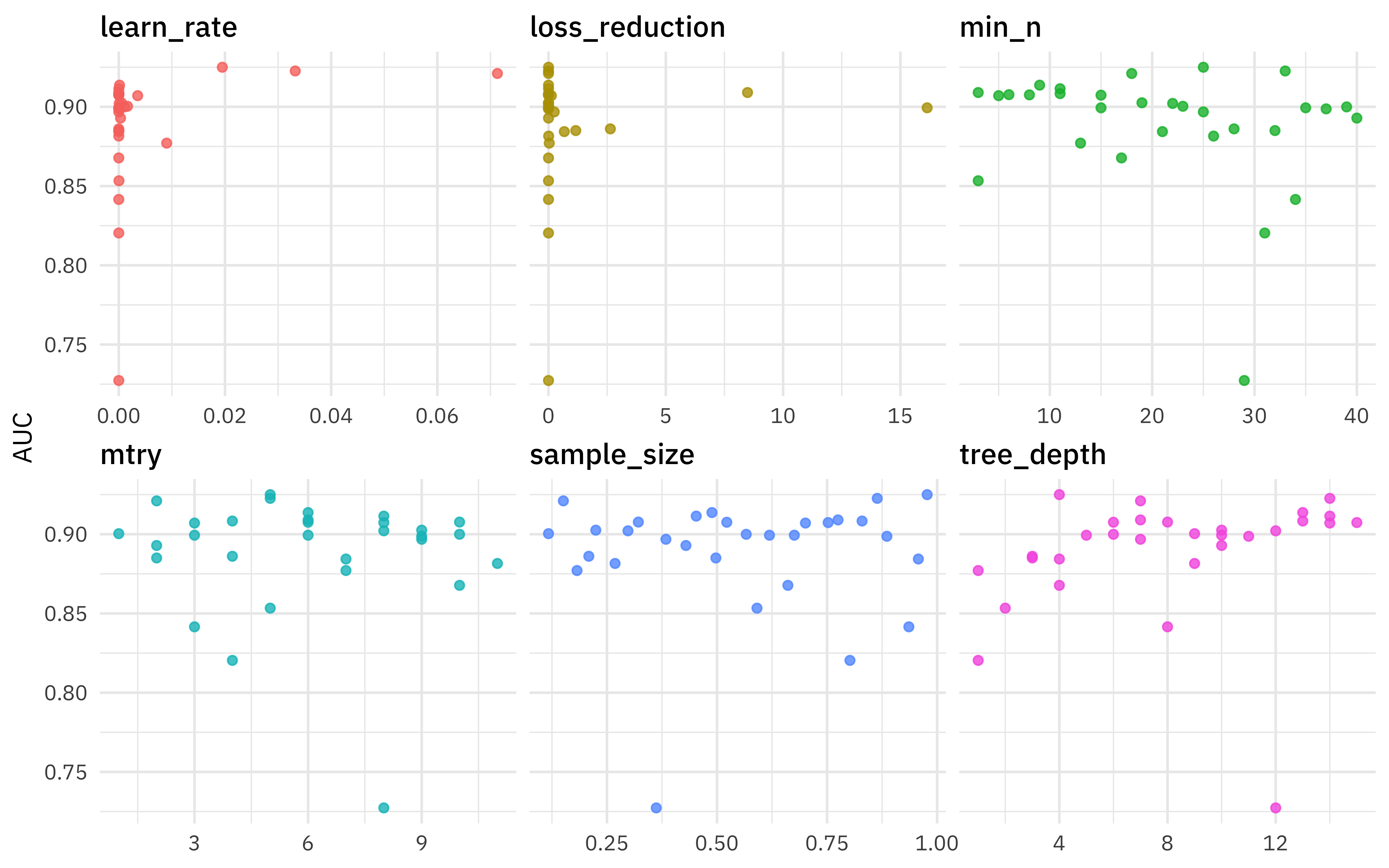
We can also use visualization to understand our results.
xgb_res %>%
  collect_metrics() %>%
  filter(.metric == "roc_auc") %>%
  select(mean, mtry:sample_size) %>%
  pivot_longer(mtry:sample_size,
               values_to = "value",
               names_to = "parameter"
  ) %>%
  ggplot(aes(value, mean, color = parameter)) +
  geom_point(alpha = 0.8, show.legend = FALSE) +
  facet_wrap(~parameter, scales = "free_x") +
  labs(x = NULL, y = "AUC")

Remember that we used a space-filling design for the parameters to try. It looks like higher values for tree depth were better, but other than that, the main thing I take away from this plot is that there are several combinations of parameters that perform well.
What are the best performing sets of parameters?
show_best(xgb_res, "roc_auc")
## # A tibble: 5 x 11
##    mtry min_n tree_depth learn_rate loss_reduction sample_size .metric
##   <int> <int>      <int>      <dbl>          <dbl>       <dbl> <chr>
## 1     5    25          4  0.0195      0.00112            0.977 roc_auc
## 2     5    33         14  0.0332      0.0000000159       0.864 roc_auc
## 3     2    18          7  0.0713      0.0000432          0.151 roc_auc
## 4     6     9         13  0.000147    0.000000191        0.488 roc_auc
## 5     8    11         14  0.0000135   0.000570           0.453 roc_auc
## # … with 4 more variables: .estimator <chr>, mean <dbl>, n <int>, std_err <dbl>
There may have been lots of parameters, but we were able to get good performance with several different combinations. Let’s choose the best one.
best_auc <- select_best(xgb_res, "roc_auc")
best_auc
## # A tibble: 1 x 6
##    mtry min_n tree_depth learn_rate loss_reduction sample_size
##   <int> <int>      <int>      <dbl>          <dbl>       <dbl>
## 1     5    25          4     0.0195        0.00112       0.977
Now let’s finalize our tuneable workflow with these parameter values.
final_xgb <- finalize_workflow(
  xgb_wf,
  best_auc
)

final_xgb
## ══ Workflow ═══════════════════════════════════════════════════════════
## Preprocessor: Formula
## Model: boost_tree()
##
## ── Preprocessor ───────────────────────────────────────────────────────
## win ~ .
##
## ── Model ──────────────────────────────────────────────────────────────
## Boosted Tree Model Specification (classification)
##
## Main Arguments:
##   mtry = 5
##   trees = 1000
##   min_n = 25
##   tree_depth = 4
##   learn_rate = 0.019501844932014
##   loss_reduction = 0.00112048286512169
##   sample_size = 0.977300804650877
##
## Computational engine: xgboost
Instead of tune() placeholders, we now have real values for all the model hyperparameters.
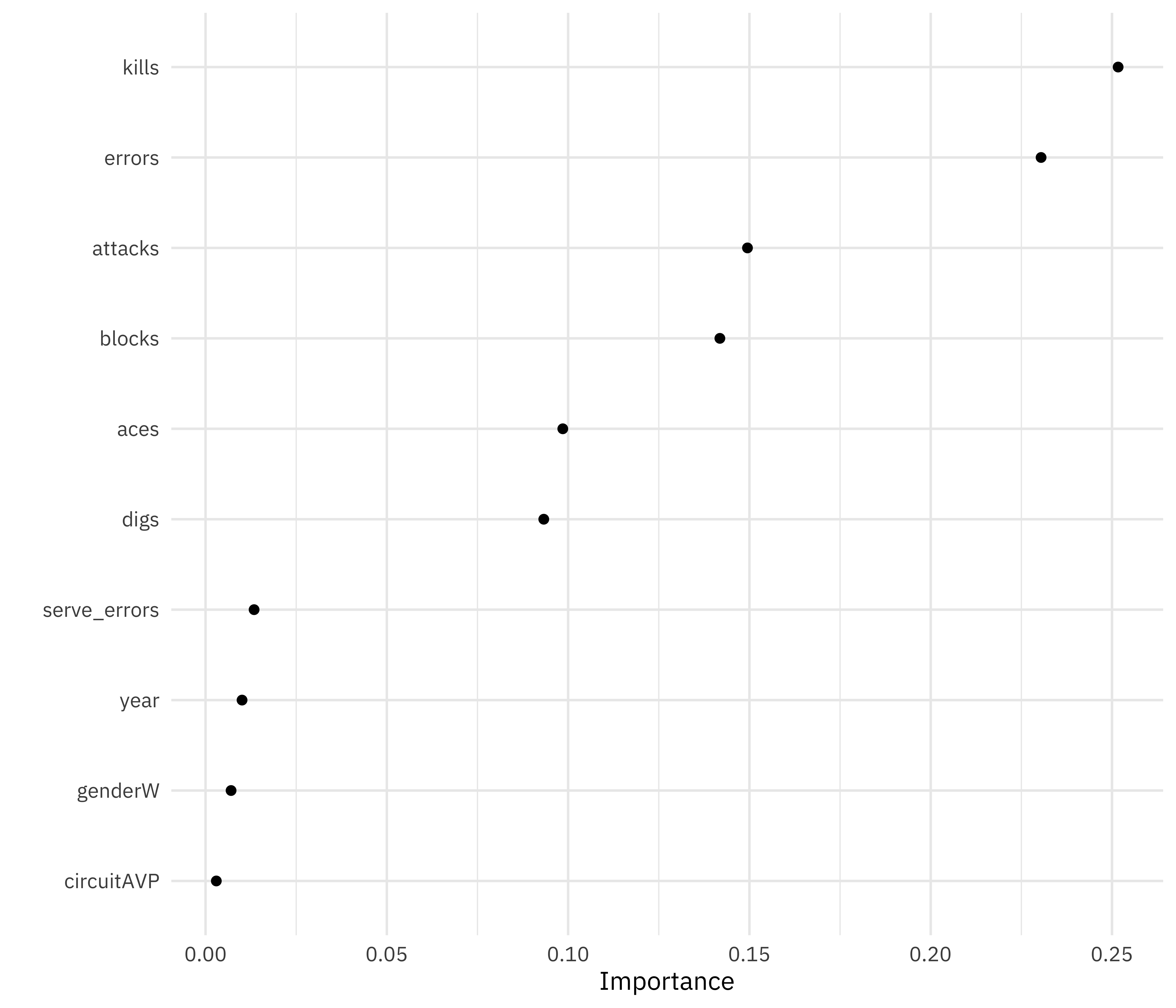
What are the most important parameters for variable importance?
library(vip)

final_xgb %>%
  fit(data = vb_train) %>%
  pull_workflow_fit() %>%
  vip(geom = "point")

The predictors that are most important in a team winning vs. losing their match are the number of kills, errors, and attacks. There is almost no difference between the two circuits, and very little difference by gender.
It’s time to go back to the testing set! Let’s use last_fit() to fit our model one last time on the training data and evaluate our model one last time on the testing set. Notice that this is the first time we have used the testing data during this whole modeling analysis.
final_res <- last_fit(final_xgb, vb_split)

collect_metrics(final_res)
## # A tibble: 2 x 3
##   .metric  .estimator .estimate
##   <chr>    <chr>          <dbl>
## 1 accuracy binary         0.843
## 2 roc_auc  binary         0.928
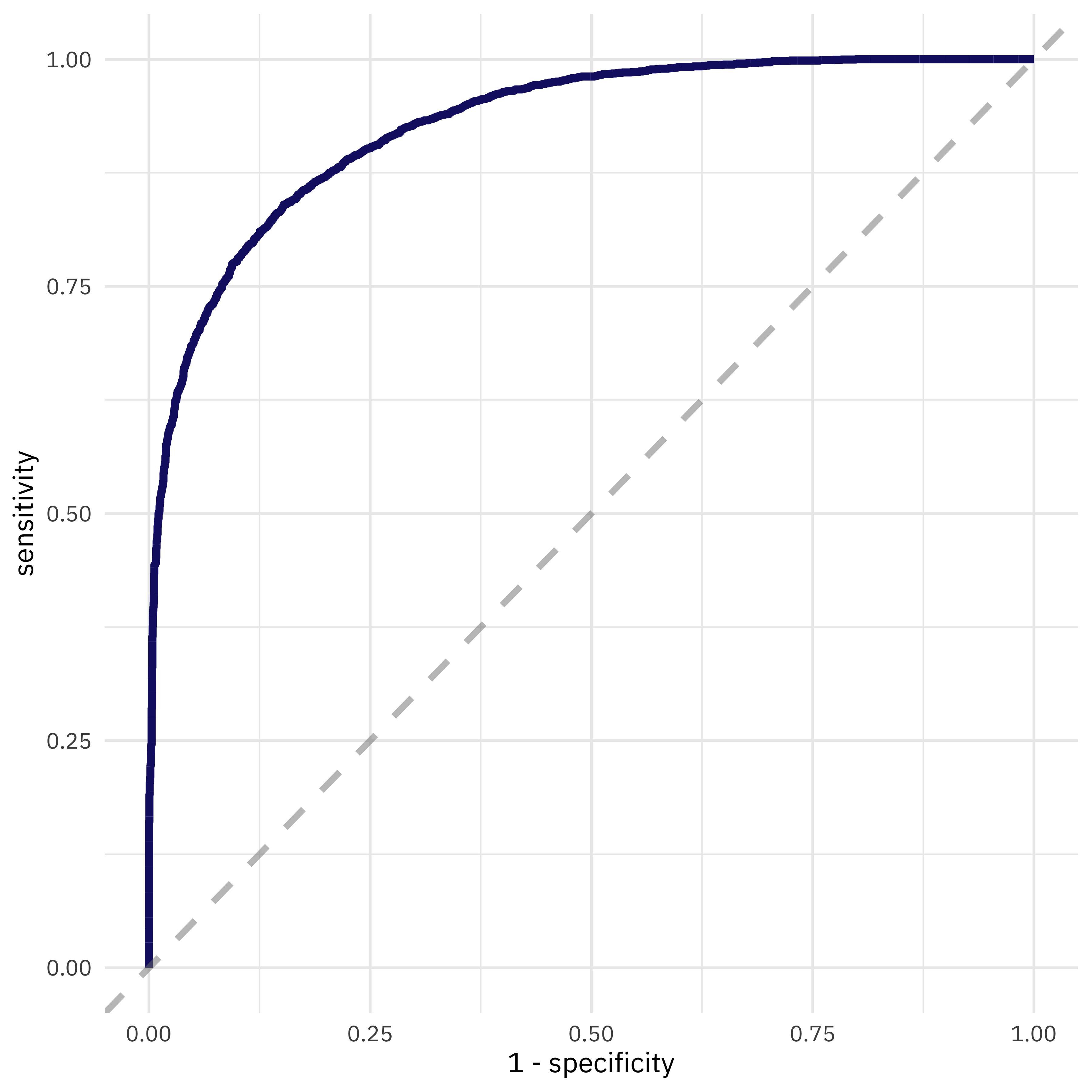
Our results here indicate that we did not overfit during the tuning process. We can also create a ROC curve for the testing set.
final_res %>%
  collect_predictions() %>%
  roc_curve(win, .pred_win) %>%
  ggplot(aes(x = 1 - specificity, y = sensitivity)) +
  geom_line(size = 1.5, color = "midnightblue") +
  geom_abline(
    lty = 2, alpha = 0.5,
    color = "gray50",
    size = 1.2
  )

- Posted on:
- May 21, 2020
- Length:
- 11 minute read, 2258 words
- Categories:
- rstats tidymodels
- Tags:
- rstats tidymodels