Amazon Alexa and Accented English
By Julia Silge
July 19, 2018
Earlier this spring, one of my data science friends here in SLC got in contact with me about some fun analysis. My friend Dylan Zwick is a founder at Pulse Labs, a voice-testing startup, and they were chatting with the Washington Post about a piece on how devices like Amazon Alexa deal with accented English. The piece is published today in the Washington Post and turned out really interesting! Let’s walk through the analysis I did for Dylan and Pulse Labs.
Understanding the data
Dylan shared voice testing results data with me via Google Sheets. The dataset included the phrase that each speaker spoke aloud, the transcription of the phrase that the Alexa device understood, and a categorization for each speaker’s accent.
library(tidyverse)
library(googlesheets)
library(stringdist)

alexa_raw <- gs_title("Alexa Speech to Text by Accent Data") %>%
    gs_read(range = cell_cols(1:4),
            verbose = FALSE) %>%
    set_names("truth", "measured", "accent", "example")
What do a few examples look like?
alexa_raw %>%
    sample_n(3) %>%
    select(truth, measured, accent) %>%
kable()| truth | measured | accent |
|---|---|---|
| China proposes removal of two term limit potentially paving way for Xi to remain President | china proposes removal of to term limit potentially paving way for gh remain president | 1 |
| As winter games close team USA falls short of expectations | ask winter games close team usa fall short of expectations | 1 |
| China proposes removal of two term limit potentially paving way for Xi to remain President | china china proposes removal of to time limit potentially paving way to remain president | 1 |
The truth column here contains the phrase that the speaker was instructed to read (there are three separate test phrases), while the measured column contains the text as it was transcribed by Alexa. The accent column is a numeric coding (1, 2, or 3) for the three categories of accented English in this text. The three categories are US flat (which would be typical broadcast English in the US, often encounted in the West and Midwest), a native speaker accent (these folks included Southern US accents and accents from Britain and Australia), and a non-native speaker accent (individuals for whom English is not their first language).
alexa <- alexa_raw %>%
    mutate(accent = case_when(accent == 1 ~ "US flat",
                              accent == 2 ~ "Native speaker accent",
                              accent == 3 ~ "Non-native speaker accent"),
           accent = factor(accent, levels = c("US flat",
                                              "Native speaker accent",
                                              "Non-native speaker accent")),
           example = case_when(example == "X" ~ TRUE,
                               TRUE ~ FALSE),
           truth = str_to_lower(truth),
           measured = str_to_lower(measured)) %>%
    filter(truth != "phrase",
           truth != "") %>%
    mutate(distance = stringdist(truth, measured, "lv"))
How many recordings from an Alexa device do we have data for, for each accent?
alexa %>%
    count(accent) %>%
kable()| accent | n |
|---|---|
| US flat | 46 |
| Native speaker accent | 33 |
| Non-native speaker accent | 20 |
This is a pretty small sample; we would be able to make stronger conclusions with more recordings.
Visualizations
Let’s look at the string distance between each between each benchmark phrase (the phrase that the speaker intended to speak) and the speech-to-text output from Alexa. We can think about this metric as the difference between what the speaker said and what Alexa heard.
alexa %>%
    ggplot(aes(accent, distance, fill = accent, color = accent)) +
    geom_boxplot(alpha = 0.2, size = 1.5) +
    labs(x = NULL, y = "String distance (Levenshtein distance)",
         title = "How well does Alexa understand different accents?",
         subtitle = "Speech with non-native accents is converted to text with the lowest accuracy") +
    theme(legend.position="none")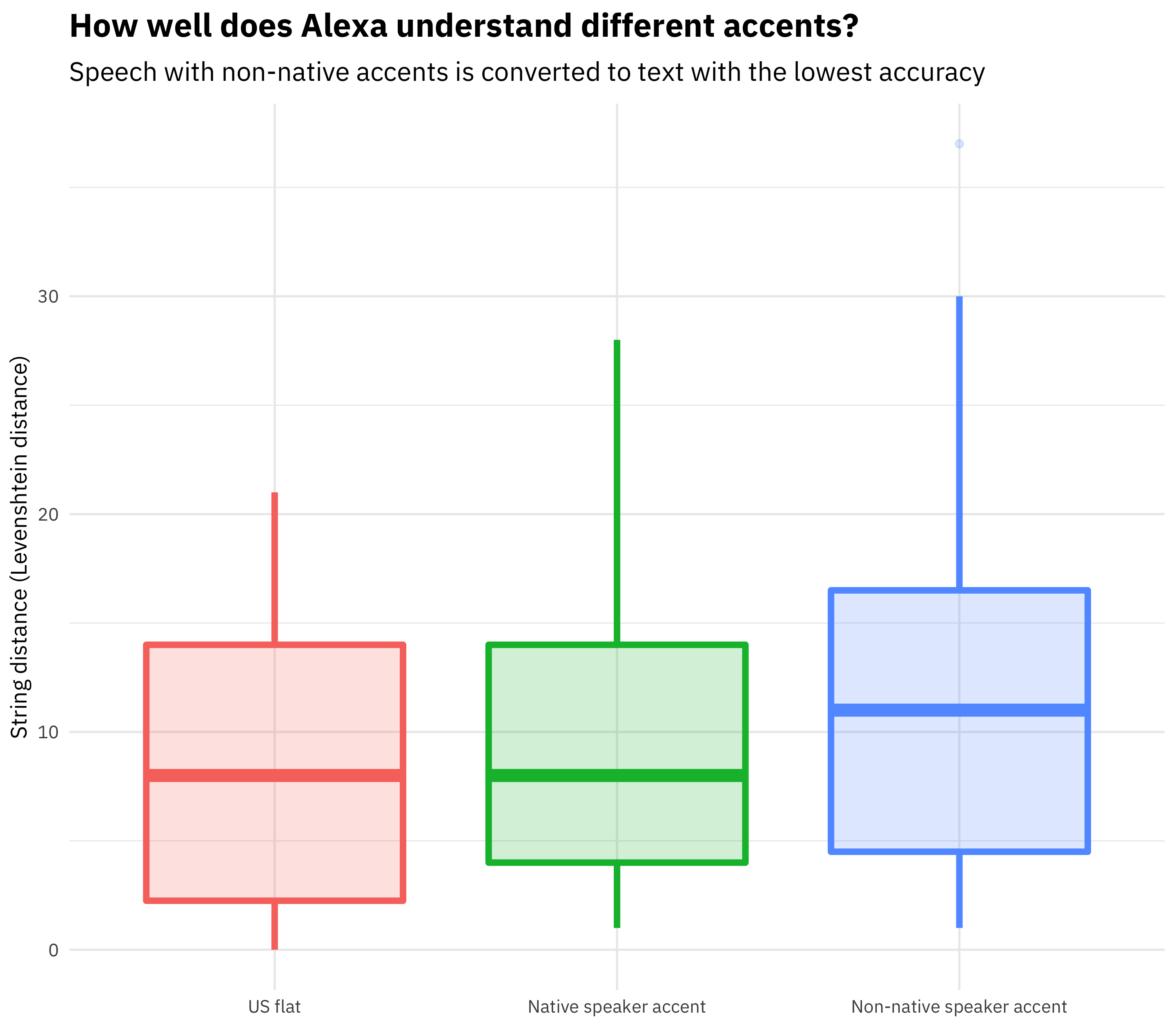
I used the Levenshtein distance, but the results are robust to other string distance measures.
alexa %>%
    group_by(accent) %>%
    summarise(distance = median(distance)) %>%
    ggplot(aes(accent, distance, fill = accent)) +
    geom_col(alpha = 0.8) +
    geom_text(aes(x = accent, y = 0.5, label = accent), color="white",
            family="IBMPlexSans-Medium", size=7, hjust = 0) +
    labs(x = NULL, y = "String distance between phrase and speech-to-text output (median Levenshtein distance)",
         title = "How well does Alexa understand English speakers with different accents?",
         subtitle = "Speech with non-native accents is converted to text with the lowest accuracy") +
    scale_y_continuous(expand = c(0,0)) +
    theme(axis.text.y=element_blank(),
          legend.position="none") +
    coord_flip()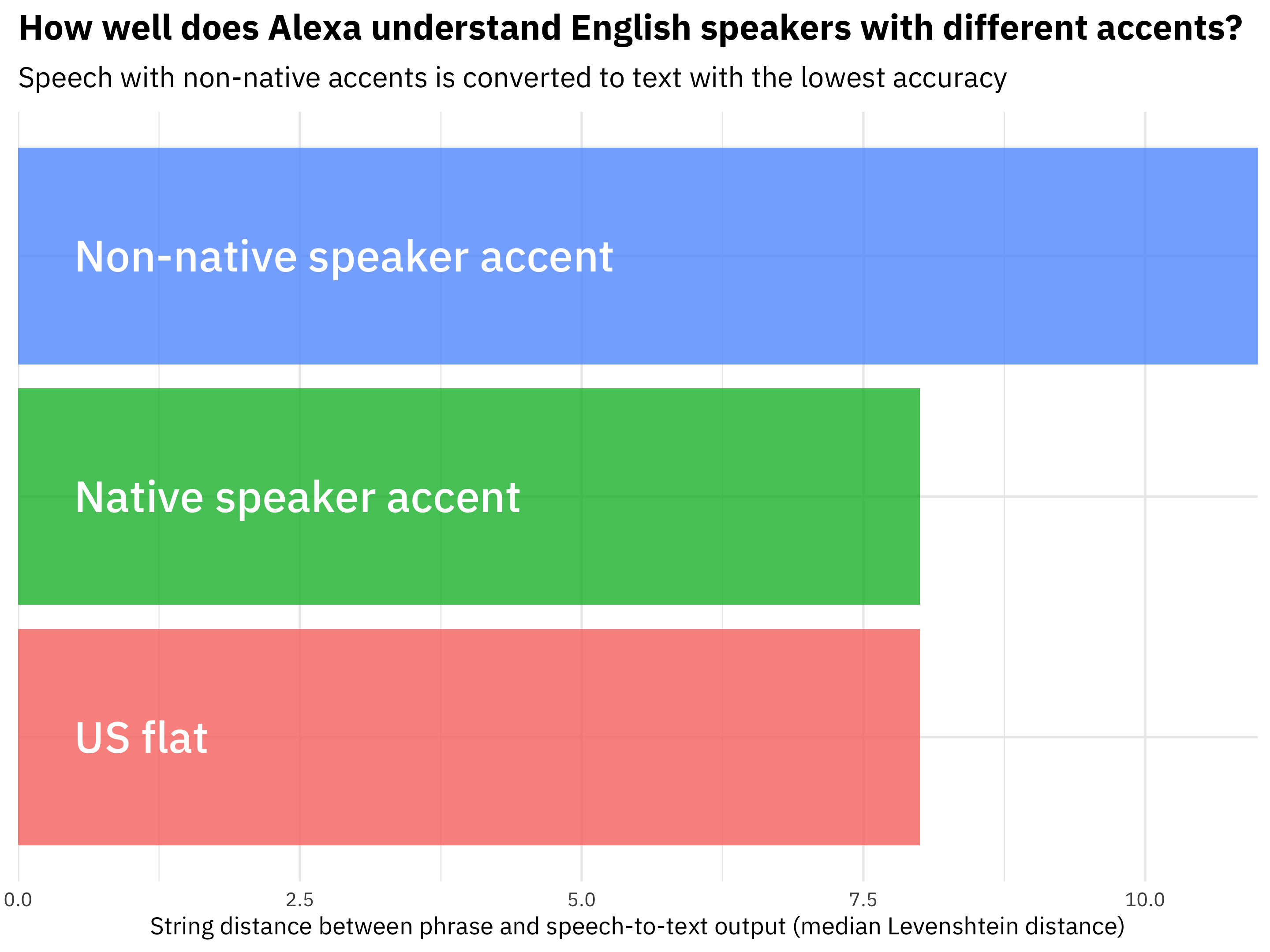
We can see here that the median difference is higher, by over 30%, for speakers with non-native-speaking accents. There is no difference for speakers with accents like British or Southern accents. That result looks pretty convincing, and certainly lines up with what other groups in the WashPo piece found, but it’s based on quite a small sample. Let’s try a statistical test.
Statistical tests
Let’s compare first the native speaker accent to the US flat group, then the non-native speakers to the US flat group.
t.test(distance ~ accent, data = alexa %>% filter(accent != "Non-native speaker accent"))##
## Welch Two Sample t-test
##
## data: distance by accent
## t = -0.55056, df = 60.786, p-value = 0.584
## alternative hypothesis: true difference in means is not equal to 0
## 95 percent confidence interval:
## -3.875468 2.202214
## sample estimates:
## mean in group US flat mean in group Native speaker accent
## 8.739130 9.575758t.test(distance ~ accent, data = alexa %>% filter(accent != "Native speaker accent"))##
## Welch Two Sample t-test
##
## data: distance by accent
## t = -1.3801, df = 25.213, p-value = 0.1797
## alternative hypothesis: true difference in means is not equal to 0
## 95 percent confidence interval:
## -8.125065 1.603326
## sample estimates:
## mean in group US flat
## 8.73913
## mean in group Non-native speaker accent
## 12.00000Performing some t-tests indicates that the group of speakers with flat accents and those with native speaker accents (Southern, British, etc.) are not different from each other; notice how big the p-value is (almost 0.6).
The situation is not clear for the comparison of the speakers with flat accents and those with non-native speaker accents, either. The p-value is about 0.18, higher than normal statistical cutoffs. It would be better to have more data to draw clear conclusions. Let’s do a simple power calculation to estimate how many measurements we would need to measure a difference this big (~30%, or ~3 on the string distance scale).
power.t.test(delta = 3, sd = sd(alexa$distance),
             sig.level = 0.05, power = 0.8)
##
## Two-sample t test power calculation
##
## n = 93.37079
## delta = 3
## sd = 7.278467
## sig.level = 0.05
## power = 0.8
## alternative = two.sided
##
## NOTE: n is number in *each* groupThis indicates we would need on the order of 90 examples per group (instead of the 20 to 40 that we have) to measure the ~30% difference we see with statistical significance. That may be a lot of voice testing to do for a single newspaper article but would be necessary to make strong statements. This dataset shows how complicated the landscape for these devices is. Check out the piece online (which includes quotes from Kaggle’s Rachael Tatman) and let me know if you have any feedback or questions!