Predict the status of #TidyTuesday Bigfoot sightings

This is the latest in my series of screencasts! I am now working on MLOps tooling full-time, and this screencast shows how to use vetiver to set up different types of prediction endpoints, using this week’s #TidyTuesday dataset on Bigfoot sightings. 🦶

Here is the code I used in the video, for those who prefer reading instead of or in addition to video.

Explore data

Our modeling goal is to predict the classification of a Bigfoot report based on the text used in the report. Let’s start by reading in the data:

library(tidyverse)
bigfoot_raw <- read_csv('https://raw.githubusercontent.com/rfordatascience/tidytuesday/master/data/2022/2022-09-13/bigfoot.csv')

bigfoot_raw %>%
  count(classification)

## # A tibble: 3 × 2
##   classification     n
##   <chr>          <int>
## 1 Class A         2481
## 2 Class B         2510
## 3 Class C           30

This dataset categorizes the reports into three classes. Class A is for clear visual sightings, Class B is for reports without a clear visual identification, and Class C is for second-hand or otherwise less reliable reports. There are very few Class C reports, so let’s only focus on Classes A and B.

bigfoot <-
  bigfoot_raw %>%
  filter(classification != "Class C", !is.na(observed)) %>%
  mutate(
    classification = case_when(
      classification == "Class A" ~ "sighting",
      classification == "Class B" ~ "possible"
    )
  )

bigfoot

## # A tibble: 4,953 × 28
##    observed  locat…¹ county state season title latit…² longi…³ date       number
##    <chr>     <chr>   <chr>  <chr> <chr>  <chr>   <dbl>   <dbl> <date>      <dbl>
##  1 "I was c…  <NA>   Winst… Alab… Summer <NA>     NA      NA   NA          30680
##  2 "Ed L. w… "East … Valde… Alas… Fall   <NA>     NA      NA   NA           1261
##  3 "While a… "Great… Washi… Rhod… Fall   Repo…    41.4   -71.5 1974-09-20   6496
##  4 "Hello, … "I wou… York … Penn… Summer <NA>     NA      NA   NA           8000
##  5 "It was … "Loggi… Yamhi… Oreg… Spring <NA>     NA      NA   NA            703
##  6 "My two … "The c… Washi… Okla… Fall   Repo…    35.3   -99.2 1973-09-28   9765
##  7 "I was s… "Vince… Washi… Ohio  Summer Repo…    39.4   -81.7 1971-08-01   4983
##  8 "Well la… "Both … Westc… New … Fall   Repo…    41.3   -73.7 2010-09-01  31940
##  9 "I grew … "The W… Washo… Neva… Fall   Repo…    39.6  -120.  1970-09-01   5692
## 10 "heh i k… "the r… Warre… New … Fall   <NA>     NA      NA   NA            438
## # … with 4,943 more rows, 18 more variables: classification <chr>,
## #   geohash <chr>, temperature_high <dbl>, temperature_mid <dbl>,
## #   temperature_low <dbl>, dew_point <dbl>, humidity <dbl>, cloud_cover <dbl>,
## #   moon_phase <dbl>, precip_intensity <dbl>, precip_probability <dbl>,
## #   precip_type <chr>, pressure <dbl>, summary <chr>, uv_index <dbl>,
## #   visibility <dbl>, wind_bearing <dbl>, wind_speed <dbl>, and abbreviated
## #   variable names ¹​location_details, ²​latitude, ³​longitude

What words from the report have the highest log odds of coming from either category?

library(tidytext)
library(tidylo)

bigfoot %>%
  unnest_tokens(word, observed) %>%
  count(classification, word) %>%
  filter(n > 100) %>%
  bind_log_odds(classification, word, n) %>%
  arrange(-log_odds_weighted)

## # A tibble: 1,747 × 4
##    classification word           n log_odds_weighted
##    <chr>          <chr>      <int>             <dbl>
##  1 possible       howl         455              14.7
##  2 sighting       fur          362              13.3
##  3 possible       heard       5397              12.7
##  4 possible       screams      327              12.5
##  5 sighting       ape          300              12.1
##  6 possible       knocks       301              12.0
##  7 sighting       hands        285              11.8
##  8 sighting       headlights   283              11.7
##  9 possible       listened     266              11.2
## 10 sighting       witness      249              11.0
## # … with 1,737 more rows

When someone has made a sighting, they see or witness a furry ape, maybe in their headlights. The reports without a clear visual sighting definitely seem like they are about sound, hearing screams and howls.

Build a model

We can start by loading the tidymodels metapackage, splitting our data into training and testing sets, and creating cross-validation samples. Think about this stage as spending your data budget.

library(tidymodels)

set.seed(123)
bigfoot_split <-
  bigfoot %>%
  select(observed, classification) %>%
  initial_split(strata = classification)

bigfoot_train <- training(bigfoot_split)
bigfoot_test <- testing(bigfoot_split)

set.seed(234)
bigfoot_folds <- vfold_cv(bigfoot_train, strata = classification)
bigfoot_folds

## #  10-fold cross-validation using stratification 
## # A tibble: 10 × 2
##    splits             id    
##    <list>             <chr> 
##  1 <split [3342/372]> Fold01
##  2 <split [3342/372]> Fold02
##  3 <split [3342/372]> Fold03
##  4 <split [3342/372]> Fold04
##  5 <split [3343/371]> Fold05
##  6 <split [3343/371]> Fold06
##  7 <split [3343/371]> Fold07
##  8 <split [3343/371]> Fold08
##  9 <split [3343/371]> Fold09
## 10 <split [3343/371]> Fold10

Next, let’s create our feature engineering recipe using word tokenization. This dataset (compared to for example modeling LEGO set names) involves much longer documents with a larger vocabulary. It is more what we would call “natural language” with English speakers using their vocabularies in typical ways, so let’s keep a pretty large number of tokens.

library(textrecipes)

bigfoot_rec <-
  recipe(classification ~ observed, data = bigfoot_train) %>%
  step_tokenize(observed) %>%
  step_tokenfilter(observed, max_tokens = 2e3) %>%
  step_tfidf(observed)

bigfoot_rec

## Recipe
## 
## Inputs:
## 
##       role #variables
##    outcome          1
##  predictor          1
## 
## Operations:
## 
## Tokenization for observed
## Text filtering for observed
## Term frequency-inverse document frequency with observed

Next let’s create a model specification for a lasso regularized logistic regression model. Lasso models can be a good choice for text data when the feature space (number of unique tokens) is big with lots of predictors. We can combine this together with the recipe in a workflow:

glmnet_spec <- 
  logistic_reg(mixture = 1, penalty = tune()) %>%
  set_engine("glmnet")

bigfoot_wf <- workflow(bigfoot_rec, glmnet_spec)

We don’t know the right amount of regularization (penalty) for this model, so we let’s tune over possible penalty values with our resamples.

doParallel::registerDoParallel()
set.seed(123)
bigfoot_res <- 
  tune_grid(
    bigfoot_wf, 
    bigfoot_folds, 
    grid = tibble(penalty = 10 ^ seq(-3, 0, by = 0.3))
  )

autoplot(bigfoot_res)

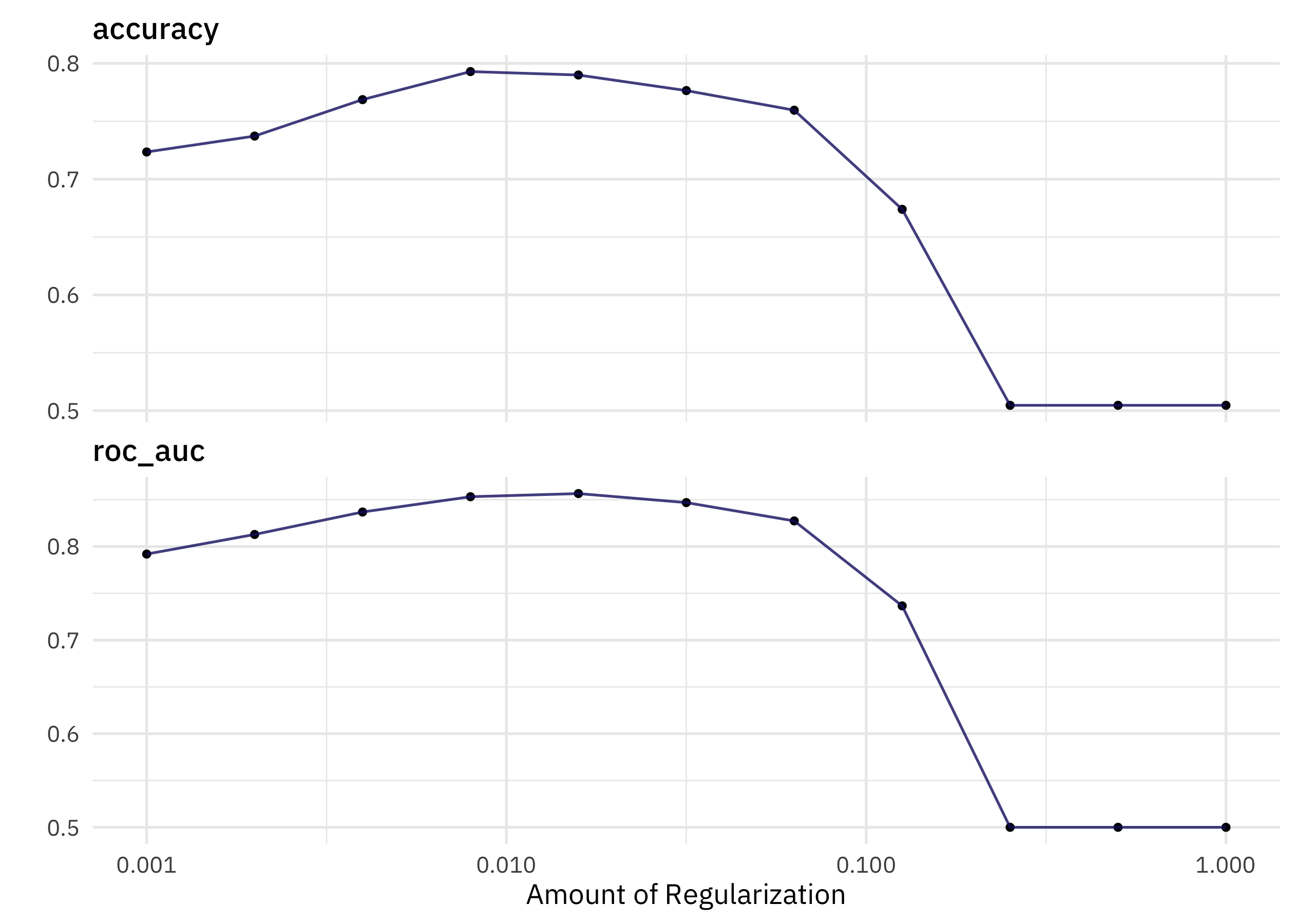
We can identify the numerically best amount of regularization:

show_best(bigfoot_res)

## # A tibble: 5 × 7
##   penalty .metric .estimator  mean     n std_err .config              
##     <dbl> <chr>   <chr>      <dbl> <int>   <dbl> <chr>                
## 1 0.0158  roc_auc binary     0.857    10 0.00463 Preprocessor1_Model05
## 2 0.00794 roc_auc binary     0.853    10 0.00545 Preprocessor1_Model04
## 3 0.0316  roc_auc binary     0.847    10 0.00487 Preprocessor1_Model06
## 4 0.00398 roc_auc binary     0.837    10 0.00675 Preprocessor1_Model03
## 5 0.0631  roc_auc binary     0.827    10 0.00506 Preprocessor1_Model07

In a case like this, we might want to choose a simpler model, i.e. a model with more regularization and fewer features (words) in it. We can identify the simplest model configuration that has performance within a certain percent loss of the numerically best one:

select_by_pct_loss(bigfoot_res, desc(penalty), metric = "roc_auc")

## # A tibble: 1 × 9
##   penalty .metric .estimator  mean     n std_err .config             .best .loss
##     <dbl> <chr>   <chr>      <dbl> <int>   <dbl> <chr>               <dbl> <dbl>
## 1  0.0316 roc_auc binary     0.847    10 0.00487 Preprocessor1_Mode… 0.857  1.13

Now let’s finalize our original tuneable workflow with this penalty value, and then fit one time to the training data and evaluate one time on the testing data.

bigfoot_final <-
  bigfoot_wf %>%
  finalize_workflow(
    select_by_pct_loss(bigfoot_res, desc(penalty), metric = "roc_auc")
  ) %>%
  last_fit(bigfoot_split)

bigfoot_final

## # Resampling results
## # Manual resampling 
## # A tibble: 1 × 6
##   splits              id               .metrics .notes   .predictions .workflow 
##   <list>              <chr>            <list>   <list>   <list>       <list>    
## 1 <split [3714/1239]> train/test split <tibble> <tibble> <tibble>     <workflow>

How did this final model do, evaluated using the testing set?

collect_metrics(bigfoot_final)

## # A tibble: 2 × 4
##   .metric  .estimator .estimate .config             
##   <chr>    <chr>          <dbl> <chr>               
## 1 accuracy binary         0.764 Preprocessor1_Model1
## 2 roc_auc  binary         0.836 Preprocessor1_Model1

We can see the model’s performance across the classes using a confusion matrix.

collect_predictions(bigfoot_final) %>%
  conf_mat(classification, .pred_class)

##           Truth
## Prediction possible sighting
##   possible      491      158
##   sighting      134      456

Let’s also check out the variables that ended up most important after regularization.

library(vip)
bigfoot_final %>%
  extract_fit_engine() %>%
  vi() 

## # A tibble: 2,000 × 3
##    Variable                  Importance Sign 
##    <chr>                          <dbl> <chr>
##  1 tfidf_observed_muscular         860. POS  
##  2 tfidf_observed_hunched          810. POS  
##  3 tfidf_observed_nose             804. POS  
##  4 tfidf_observed_shaggy           779. POS  
##  5 tfidf_observed_guessing         768. POS  
##  6 tfidf_observed_whooping         716. NEG  
##  7 tfidf_observed_especially       682. NEG  
##  8 tfidf_observed_putting          673. POS  
##  9 tfidf_observed_literally        664. NEG  
## 10 tfidf_observed_admit            621. POS  
## # … with 1,990 more rows

Here again, we see the words about seeing vs. hearing Bigfoot.

Deploy the model

The first step to deploy this model is to create a deployable model object with vetiver.

library(vetiver)
v <- bigfoot_final %>%
  extract_workflow() %>%
  vetiver_model("bigfoot")
v

## 
## ── bigfoot ─ <butchered_workflow> model for deployment 
## A glmnet classification modeling workflow using 1 feature

The typical next steps is to version your model, but for this blog post, let’s go straight to how we would make predictions. We can use predict() or augment() with our deployable model object:

augment(v, slice_sample(bigfoot_test, n = 10))

## # A tibble: 10 × 5
##    observed                                      class…¹ .pred…² .pred…³ .pred…⁴
##    <chr>                                         <chr>   <fct>     <dbl>   <dbl>
##  1 "My husband, myself and my husbands friend w… possib… possib…  0.776    0.224
##  2 "We live about a mile from Austin Bridge Roa… sighti… sighti…  0.211    0.789
##  3 "Hello my name  is **** and I have a story. … sighti… sighti…  0.198    0.802
##  4 "On November 7th and 8th I re-visited my fam… possib… possib…  0.592    0.408
##  5 "I am a tree trimmer in Ohio and today 1-2-1… possib… possib…  0.518    0.482
##  6 "My wife and I were returning from TMT Farms… sighti… sighti…  0.0785   0.922
##  7 "Bigfoot sighting. Late March or early April… sighti… sighti…  0.407    0.593
##  8 "Preface:  The following is an excerpt from … possib… possib…  0.551    0.449
##  9 "Found a fresh footprint approximately 18\" … possib… possib…  0.631    0.369
## 10 "A neighbor's chicken coop was raided. I kee… possib… sighti…  0.382    0.618
## # … with abbreviated variable names ¹​classification, ²​.pred_class,
## #   ³​.pred_possible, ⁴​.pred_sighting

To deploy this model elsewhere away from my local machine, I would set up a REST API. You can specify what kind of predictions to make when you create that API. I can set up an API to make the default predictions (type = "class" would be the default in this case for tidymodels):

library(plumber)
## pipe this to `pr_run()`
pr() %>% 
  vetiver_api(v)

## # Plumber router with 2 endpoints, 4 filters, and 1 sub-router.
## # Use `pr_run()` on this object to start the API.
## ├──[queryString]
## ├──[body]
## ├──[cookieParser]
## ├──[sharedSecret]
## ├──/logo
## │  │ # Plumber static router serving from directory: /Library/Frameworks/R.framework/Versions/4.2-arm64/Resources/library/vetiver
## ├──/ping (GET)
## └──/predict (POST)

If I want to specify an argument to control the type of predictions, like returning probabilities instead of the predicted class, I can do that instead:

## pipe this to `pr_run()`
pr() %>% 
  vetiver_api(v, type = "prob")

## # Plumber router with 2 endpoints, 4 filters, and 1 sub-router.
## # Use `pr_run()` on this object to start the API.
## ├──[queryString]
## ├──[body]
## ├──[cookieParser]
## ├──[sharedSecret]
## ├──/logo
## │  │ # Plumber static router serving from directory: /Library/Frameworks/R.framework/Versions/4.2-arm64/Resources/library/vetiver
## ├──/ping (GET)
## └──/predict (POST)

We would generally recommend that these kinds of decisions are made at the API or endpoint level, e.g. set up a single endpoint for a single type of prediction. However, you could write custom code so arguments like the type of prediction are passed in as query parameters if you wish.