Find high FREX and high lift words for #TidyTuesday Stranger Things dialogue
By Julia Silge in rstats
October 20, 2022
This is the latest in my series of
screencasts! This screencast demonstrates how to use some brand-new functionality in
tidytext, using this week’s
#TidyTuesday dataset on Stranger Things. 👻
The code in this blog post requires the GitHub version of tidytext as of publication. Here is the code I used in the video, for those who prefer reading instead of or in addition to video.
Explore data
Our modeling goal is to “discover” topics in Stranger Things dialogue. Instead of a supervised or predictive model where our observations have labels, this is an unsupervised approach. Let’s start by reading in the data, and focusing only on the show’s dialogue:
library(tidyverse)
episodes_raw <- read_csv('https://raw.githubusercontent.com/rfordatascience/tidytuesday/master/data/2022/2022-10-18/stranger_things_all_dialogue.csv')

dialogue <-
  episodes_raw %>%
  filter(!is.na(dialogue)) %>%
  mutate(season = paste0("season", season))

dialogue
## # A tibble: 26,041 × 8
## season episode line raw_text stage…¹ dialo…² start…³ end_t…⁴
## <chr> <dbl> <dbl> <chr> <chr> <chr> <time> <time>
## 1 season1 1 9 [Mike] Something is co… [Mike] Someth… 01'44" 01'48"
## 2 season1 1 10 A shadow grows on the … <NA> A shad… 01'48" 01'52"
## 3 season1 1 11 -It is almost here. -W… <NA> It is … 01'52" 01'54"
## 4 season1 1 12 What if it's the Demog… <NA> What i… 01'54" 01'56"
## 5 season1 1 13 Oh, Jesus, we're so sc… <NA> Oh, Je… 01'56" 01'59"
## 6 season1 1 14 It's not the Demogorgo… <NA> It's n… 01'59" 02'00"
## 7 season1 1 15 An army of troglodytes… <NA> An arm… 02'00" 02'02"
## 8 season1 1 16 -Troglodytes? -Told ya… [chuck… Troglo… 02'02" 02'05"
## 9 season1 1 18 [softly] Wait a minute. [softl… Wait a… 02'08" 02'09"
## 10 season1 1 19 Did you hear that? <NA> Did yo… 02'10" 02'12"
## # … with 26,031 more rows, and abbreviated variable names ¹stage_direction,
## # ²dialogue, ³start_time, ⁴end_time
To start out with, let’s create a tidy, tokenized version of the dialogue.
library(tidytext)

tidy_dialogue <-
  dialogue %>%
  unnest_tokens(word, dialogue)

tidy_dialogue
## # A tibble: 143,885 × 8
## season episode line raw_text stage…¹ start…² end_t…³ word
## <chr> <dbl> <dbl> <chr> <chr> <time> <time> <chr>
## 1 season1 1 9 [Mike] Something is comi… [Mike] 01'44" 01'48" some…
## 2 season1 1 9 [Mike] Something is comi… [Mike] 01'44" 01'48" is
## 3 season1 1 9 [Mike] Something is comi… [Mike] 01'44" 01'48" comi…
## 4 season1 1 9 [Mike] Something is comi… [Mike] 01'44" 01'48" some…
## 5 season1 1 9 [Mike] Something is comi… [Mike] 01'44" 01'48" hung…
## 6 season1 1 9 [Mike] Something is comi… [Mike] 01'44" 01'48" for
## 7 season1 1 9 [Mike] Something is comi… [Mike] 01'44" 01'48" blood
## 8 season1 1 10 A shadow grows on the wa… <NA> 01'48" 01'52" a
## 9 season1 1 10 A shadow grows on the wa… <NA> 01'48" 01'52" shad…
## 10 season1 1 10 A shadow grows on the wa… <NA> 01'48" 01'52" grows
## # … with 143,875 more rows, and abbreviated variable names ¹stage_direction,
## # ²start_time, ³end_time
What words from the dialogue have the highest log odds of coming from each season?
library(tidylo)

tidy_dialogue %>%
  count(season, word, sort = TRUE) %>%
  bind_log_odds(season, word, n) %>%
  filter(n > 20) %>%
  group_by(season) %>%
  slice_max(log_odds_weighted, n = 10) %>%
  mutate(word = reorder_within(word, log_odds_weighted, season)) %>%
  ggplot(aes(log_odds_weighted, word, fill = season)) +
  geom_col(show.legend = FALSE) +
  facet_wrap(vars(season), scales = "free") +
  scale_y_reordered() +
  labs(y = NULL)
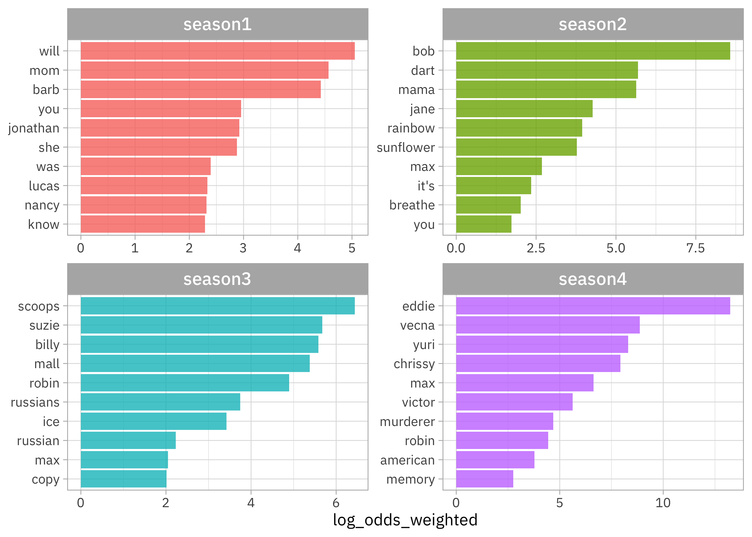
We can see that:
- Season 1 is more about Barb 😭 and Will
- Season 2 introduces Bob 😭😭, Dart, and the rainbow/sunflower imagery
- Season 3 has Russians and the Scoops shop
- Season 4 brings us Eddie, Vecna, and Yuri
Lots of proper nouns in here!
Train a topic model
To train a topic model with the stm package, we need to create a sparse matrix from our tidy tibble of tokens. Let’s treat each episode of Stranger Things as a document.
dialogue_sparse <-
  tidy_dialogue %>%
  mutate(document = paste(season, episode, sep = "_")) %>%
  count(document, word) %>%
  filter(n > 5) %>%
  cast_sparse(document, word, n)

dim(dialogue_sparse)
## [1] 34 562
This means there are 34 episodes (i.e. documents) and 562 different tokens (i.e. terms or words) in our dataset for modeling.
A topic model like this one models:
- each document as a mixture of topics
- each topic as a mixture of words
The most important parameter when training a topic modeling is K, the number of topics. This is like k in k-means in that it is a hyperparamter of the model and we must choose this value ahead of time. We could
try multiple different values to find the best value for K, but this is a pretty small dataset so let’s just stick with K = 5.
library(stm)
set.seed(123)
topic_model <- stm(dialogue_sparse, K = 5, verbose = FALSE)
To get a quick view of the results, we can use summary().
summary(topic_model)
## A topic model with 5 topics, 34 documents and a 562 word dictionary.

## Topic 1 Top Words:
##       Highest Prob: you, i, the, to, a, and, it
##       FREX: max, mean, they're, i'm, don't, i, know
##       Lift: clarke, dart, soon, better, girlfriend, late, living
##       Score: girlfriend, max, dart, duck, mr, building, kline's
## Topic 2 Top Words:
##       Highest Prob: you, i, the, a, to, it, and
##       FREX: he's, let, we, he, go, us, what
##       Lift: flayer, party, fact, flayed, children, hold, tied
##       Score: flayer, ice, cherry, says, bob, key, code
## Topic 3 Top Words:
##       Highest Prob: you, i, the, to, a, and, that
##       FREX: eddie, as, only, chrissy, make, has, much
##       Lift: ray, california, dad, deal, hellfire, mrs, tonight
##       Score: ray, eddie, only, chrissy, try, had, vecna
## Topic 4 Top Words:
##       Highest Prob: you, i, the, to, it, a, and
##       FREX: go, mike, come, jonathan, on, okay, get
##       Lift: jonathan, gone, jingle, kids, terry, answer, blood
##       Score: christmas, jonathan, copy, jingle, gone, bell, scoops
## Topic 5 Top Words:
##       Highest Prob: you, i, the, to, a, what, it
##       FREX: will, mom, lucas, murderer, barb, he, know
##       Lift: byers, else, upside, fourfifty, demogorgon, lonnie, shut
##       Score: threeonefive, mom, barb, lucas, murderer, hopper, sunflower
Explore topic model results
To explore more deeply, we can tidy() the topic model results to get a dataframe that we can compute on. The "beta" matrix of topic-word probabilities gives us the highest probability words from each topic.
tidy(topic_model, matrix = "beta") %>%
  group_by(topic) %>%
  slice_max(beta, n = 10, ) %>%
  mutate(rank = row_number()) %>%
  ungroup() %>%
  select(-beta) %>%
  pivot_wider(
    names_from = "topic",
    names_glue = "topic {.name}",
    values_from = term
  ) %>%
  select(-rank) %>%
  knitr::kable()
| topic 1 | topic 2 | topic 3 | topic 4 | topic 5 |
|---|---|---|---|---|
| you | you | you | you | you |
| i | i | i | i | i |
| the | the | the | the | the |
| to | a | to | to | to |
| a | to | a | it | a |
| and | it | and | a | what |
| it | and | that | and | it |
| that | what | it | is | and |
| what | that | is | go | that |
| it’s | we | we | this | is |
Well, that’s pretty boring, isn’t it?! This can happen a lot with topic modeling; you typically don’t want to remove stop words before building topic models but then the highest probability words look mostly the same from each topic.
People who work with topic models have come up with alternate metrics for identifying important words. One is FREX (high frequency and high exclusivity) and another is lift. Look at the details at ?stm::calcfrex() and ?stm::calclift() to learn more about these metrics, but they measure about what they sound like they do.
Before now, there was no support in tidytext for these alternate ways of identifying important words, but I just merged in new functionality for this. To use these as of today, you will need to install from GitHub via devtools::install_github("juliasilge/tidytext").
We can find high FREX words:
tidy(topic_model, matrix = "frex") %>%
  group_by(topic) %>%
  slice_head(n = 10) %>%
  mutate(rank = row_number()) %>%
  ungroup() %>%
  pivot_wider(
    names_from = "topic",
    names_glue = "topic {.name}",
    values_from = term
  ) %>%
  select(-rank) %>%
  knitr::kable()
| topic 1 | topic 2 | topic 3 | topic 4 | topic 5 |
|---|---|---|---|---|
| red | cops | billy | night | life |
| running | enzo | cherry | because | anything |
| lucas | billy | says | mike | much |
| thought | suzie | house | say | too |
| byers | ghostbusters | building | dart | after |
| max | son | men | wait | off |
| holy | hi | two | last | nina |
| nina | wait | girl | move | old |
| eleven | talking | eddie | am | their |
| hell | um | jesus | wanna | them |
Or high lift words:
tidy(topic_model, matrix = "lift") %>%
  group_by(topic) %>%
  slice_head(n = 10) %>%
  mutate(rank = row_number()) %>%
  ungroup() %>%
  pivot_wider(
    names_from = "topic",
    names_glue = "topic {.name}",
    values_from = term
  ) %>%
  select(-rank) %>%
  knitr::kable()
| topic 1 | topic 2 | topic 3 | topic 4 | topic 5 |
|---|---|---|---|---|
| clarke | flayer | ray | jonathan | byers |
| dart | party | california | gone | else |
| soon | fact | dad | jingle | upside |
| better | flayed | deal | kids | fourfifty |
| girlfriend | children | hellfire | terry | demogorgon |
| late | hold | mrs | answer | lonnie |
| living | tied | tonight | blood | shut |
| sir | illinois | might | christmas | barb |
| mistakes | machina | prison | merry | chug |
| shadow | smirnoff | step | telling | missing |
These return a ranked set of words (not the underlying metrics themselves). They give us a much clearer idea of what makes each topic unique!
To connect the topics back to seasons, let’s use tidy() again, finding the "gamma" matrix of document-topic probabilities.
episode_gamma <- tidy(
  topic_model,
  matrix = "gamma",
  document_names = rownames(dialogue_sparse)
)
episode_gamma
## # A tibble: 170 × 3
##    document  topic    gamma
##    <chr>     <int>    <dbl>
##  1 season1_1     1 0.000817
##  2 season1_2     1 0.000749
##  3 season1_3     1 0.00104
##  4 season1_4     1 0.000758
##  5 season1_5     1 0.000806
##  6 season1_6     1 0.00201
##  7 season1_7     1 0.00125
##  8 season1_8     1 0.000633
##  9 season2_1     1 0.800
## 10 season2_2     1 0.516
## # … with 160 more rows
We can parse these results to find the season info again:
episodes_parsed <-
  episode_gamma %>%
  separate(document, c("season", "episode"), sep = "_")

episodes_parsed
## # A tibble: 170 × 4
##    season  episode topic    gamma
##    <chr>   <chr>   <int>    <dbl>
##  1 season1 1           1 0.000817
##  2 season1 2           1 0.000749
##  3 season1 3           1 0.00104
##  4 season1 4           1 0.000758
##  5 season1 5           1 0.000806
##  6 season1 6           1 0.00201
##  7 season1 7           1 0.00125
##  8 season1 8           1 0.000633
##  9 season2 1           1 0.800
## 10 season2 2           1 0.516
## # … with 160 more rows
Let’s visualize how these document-topic probabilities are distributed over the seasons.
episodes_parsed %>%
    mutate(topic = factor(topic)) %>%
    ggplot(aes(topic, gamma, fill = topic)) +
    geom_boxplot(alpha = 0.7, show.legend = FALSE) +
    facet_wrap(vars(season)) +
    labs(y = expression(gamma))
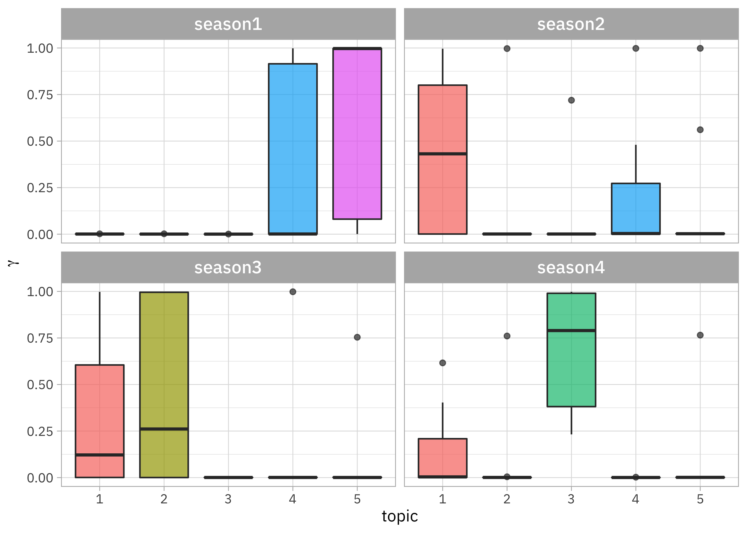
Each season mostly consists of one of these topics, with season 3 consisting of more like two topics. We could also look at how topic is related to season by using stm::estimateEffect(), like
in this blog post.