Use Docker to deploy a model for #TidyTuesday LEGO sets

This is the latest in my series of screencasts! Like I said last time, I am stepping away from working on tidymodels to focus on MLOps tools full-time, and this screencast shows how to use vetiver to deploy a model with Docker, using this week’s #TidyTuesday dataset on LEGO sets.

Here is the code I used in the video, for those who prefer reading instead of or in addition to video.

Load data

Our modeling goal is to predict how many pieces there are in a LEGO set based on the set’s name. The model itself is probably not going to perform super well (it’s a little silly) but we can use it as a way to demonstrate deploying such a model in a Docker container. Let’s start by reading in the data:

library(tidyverse)
lego_sets <- read_csv('https://raw.githubusercontent.com/rfordatascience/tidytuesday/master/data/2022/2022-09-06/sets.csv.gz')
glimpse(lego_sets)

## Rows: 19,798
## Columns: 6
## $ set_num   <chr> "001-1", "0011-2", "0011-3", "0012-1", "0013-1", "0014-1", "…
## $ name      <chr> "Gears", "Town Mini-Figures", "Castle 2 for 1 Bonus Offer", …
## $ year      <dbl> 1965, 1979, 1987, 1979, 1979, 1979, 1979, 1979, 1965, 2013, …
## $ theme_id  <dbl> 1, 67, 199, 143, 143, 143, 143, 189, 1, 497, 366, 366, 366, …
## $ num_parts <dbl> 43, 12, 0, 12, 12, 12, 18, 15, 3, 4, 403, 35, 0, 0, 57, 77, …
## $ img_url   <chr> "https://cdn.rebrickable.com/media/sets/001-1.jpg", "https:/…

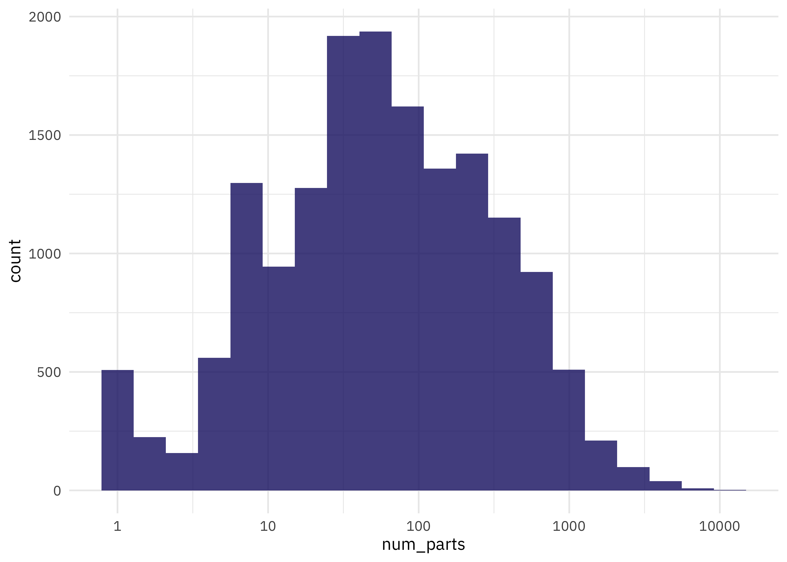
How are the number of LEGO parts per set distributed?

lego_sets %>%
    filter(num_parts > 0) %>%
    ggplot(aes(num_parts)) +
    geom_histogram(bins = 20) +
    scale_x_log10()

Build a model

We can start by loading the tidymodels metapackage, splitting our data into training and testing sets, and creating cross-validation samples. Think about this stage as spending your data budget.

library(tidymodels)

set.seed(123)
lego_split <- lego_sets %>%
    filter(num_parts > 0) %>%
    transmute(num_parts = log10(num_parts), name) %>%
    initial_split(strata = num_parts)

lego_train <- training(lego_split)
lego_test <- testing(lego_split)

set.seed(234)
lego_folds <- vfold_cv(lego_train, strata = num_parts)
lego_folds

## #  10-fold cross-validation using stratification 
## # A tibble: 10 × 2
##    splits               id    
##    <list>               <chr> 
##  1 <split [10911/1214]> Fold01
##  2 <split [10911/1214]> Fold02
##  3 <split [10911/1214]> Fold03
##  4 <split [10911/1214]> Fold04
##  5 <split [10913/1212]> Fold05
##  6 <split [10913/1212]> Fold06
##  7 <split [10913/1212]> Fold07
##  8 <split [10914/1211]> Fold08
##  9 <split [10914/1211]> Fold09
## 10 <split [10914/1211]> Fold10

Next, let’s create our feature engineering recipe using basic word tokenization and keeping only the top 200 words used most in LEGO set names.

library(textrecipes)

lego_rec <- recipe(num_parts ~ name, data = lego_train) %>%
    step_tokenize(name) %>%
    step_tokenfilter(name, max_tokens = 200) %>%
    step_tfidf(name)

lego_rec

## Recipe
## 
## Inputs:
## 
##       role #variables
##    outcome          1
##  predictor          1
## 
## Operations:
## 
## Tokenization for name
## Text filtering for name
## Term frequency-inverse document frequency with name

Next let’s create a model specification for a linear support vector machine. Linear SVMs are often a good starting choice for text models. We can combine this together with the recipe in a workflow:

svm_spec <- svm_linear(mode = "regression")
lego_wf <- workflow(lego_rec, svm_spec)

Now let’s fit this workflow (that combines feature engineering with the SVM model) to the resamples we created earlier. We do this so we can have a reliable estimate of our model’s performance before we deploy it.

set.seed(234)

doParallel::registerDoParallel()
lego_rs <- fit_resamples(lego_wf, lego_folds)
collect_metrics(lego_rs)

## # A tibble: 2 × 6
##   .metric .estimator  mean     n std_err .config             
##   <chr>   <chr>      <dbl> <int>   <dbl> <chr>               
## 1 rmse    standard   0.675    10 0.00370 Preprocessor1_Model1
## 2 rsq     standard   0.185    10 0.00497 Preprocessor1_Model1

Like we expected with this somewhat silly modeling approach, we don’t get extraordinary performance. The R^2, for example, indicates that we don’t explain much of the variation in number of parts per set by the name. Nonetheless, let’s fit our model on last time to the whole training set at once (rather than resampled data) and evaluate on the testing set. This is the first time we have touched the testing set.

final_fitted <- last_fit(lego_wf, lego_split)
collect_metrics(final_fitted)

## # A tibble: 2 × 4
##   .metric .estimator .estimate .config             
##   <chr>   <chr>          <dbl> <chr>               
## 1 rmse    standard       0.681 Preprocessor1_Model1
## 2 rsq     standard       0.176 Preprocessor1_Model1

Since this is a linear model, let’s look at the coefficients. What words are associated with higher numbers of LEGO parts?

final_fitted %>%
    extract_workflow() %>%
    tidy() %>%
    arrange(-estimate)

## # A tibble: 201 × 2
##    term                 estimate
##    <chr>                   <dbl>
##  1 Bias                    1.71 
##  2 tfidf_name_challenge    0.207
##  3 tfidf_name_castle       0.175
##  4 tfidf_name_cargo        0.161
##  5 tfidf_name_calendar     0.157
##  6 tfidf_name_hogwarts     0.155
##  7 tfidf_name_bucket       0.154
##  8 tfidf_name_shuttle      0.153
##  9 tfidf_name_house        0.151
## 10 tfidf_name_mech         0.150
## # … with 191 more rows
## # ℹ Use `print(n = ...)` to see more rows

Buckets and castles have lots of pieces!

Version and deploy the model

Let’s use the same extract_workflow() helper to create a deployable model object with vetiver:

library(vetiver)

v <- final_fitted %>%
    extract_workflow() %>%
    vetiver_model(model_name = "lego-sets")
v

## 
## ── lego-sets ─ <butchered_workflow> model for deployment 
## A LiblineaR regression modeling workflow using 1 feature

This object has everything we need to deploy our model in a new computer environment, like the Docker container we are about to make.

The next step is to store and version the model object somewhere. I’ll use RStudio Connect as my “board”, but you could also store your model object somewhere else like S3 or Azure’s blob storage. You can store your model anywhere, as long as the Docker container can authenticate to where it is stored.

library(pins)
board <- board_rsconnect()
board %>% vetiver_pin_write(v)

I’m going to generate two files now, a Plumber file that will get copied over to the Docker container and a Dockerfile.

vetiver_write_plumber(board, "julia.silge/lego-sets", rsconnect = FALSE)
vetiver_write_docker(v)

## * Lockfile written to 'vetiver_renv.lock'.

Technically I generated three files here; vetiver_write_docker() also creates a vetiver_renv.lock file that says exactly which versions of the packages I need to deploy my model. What does the Dockerfile look like?

## # Generated by the vetiver package; edit with care
## 
## FROM rocker/r-ver:4.2.1
## ENV RENV_CONFIG_REPOS_OVERRIDE https://packagemanager.rstudio.com/cran/latest
## 
## RUN apt-get update -qq && apt-get install -y --no-install-recommends \
##   libcurl4-openssl-dev \
##   libicu-dev \
##   libsodium-dev \
##   libssl-dev \
##   make
## 
## COPY vetiver_renv.lock renv.lock
## RUN Rscript -e "install.packages('renv')"
## RUN Rscript -e "renv::restore()"
## COPY plumber.R /opt/ml/plumber.R
## EXPOSE 8000
## ENTRYPOINT ["R", "-e", "pr <- plumber::plumb('/opt/ml/plumber.R'); pr$run(host = '0.0.0.0', port = 8000)"]

This Dockerfile helps us build a new, separate computational environment that the model can be served from. Now that I need to build the Dockerfile, I will move out of R and work on the command line. Since I am on an M1 Mac but the public RSPM I am using builds R packages for Intel chips, I will use a special --platform option to force the Docker container to build for non-ARM architecture.

docker build --platform linux/amd64 -t lego-set-names .

The Docker container needs to authenticate to where my model pin exists (RStudio Connect in this case) so I will run the container and pass an .Renviron file with my Connect credentials:

docker run --env-file .Renviron --rm -p 8000:8000 lego-set-names

A file of environment variables for Docker should not have quotes around the variables; this is different than environment variables for R, which can have quotes. Specify your variables in this file like CONNECT_SERVER=https://colorado.rstudio.com/rsc/.

Now my Docker container is running and I can visit it at, in my case, http://127.0.0.1:8000/__docs__/. You can see how I interacted with the visual documentation in the screencast, and Docker containers like these can be deployed in many different ways, from using your own servers to the cloud platforms.