Hyperparameter tuning and #TidyTuesday food consumption

Last week I published a screencast demonstrating how to use the tidymodels framework and specifically the recipes package. Today, I’m using this week’s #TidyTuesday dataset on food consumption around the world to show hyperparameter tuning!

Here is the code I used in the video, for those who prefer reading instead of or in addition to video.

Explore the data

Our modeling goal here is to predict which countries are Asian countries and which countries are not, based on their patterns of food consumption in the eleven categories from the #TidyTuesday dataset. The original data is in a long, tidy format, and includes information on the carbon emission associated with each category of food consumption.

library(tidyverse)

food_consumption <- readr::read_csv("https://raw.githubusercontent.com/rfordatascience/tidytuesday/master/data/2020/2020-02-18/food_consumption.csv")

food_consumption

## # A tibble: 1,430 x 4
##    country   food_category            consumption co2_emmission
##    <chr>     <chr>                          <dbl>         <dbl>
##  1 Argentina Pork                           10.5          37.2
##  2 Argentina Poultry                        38.7          41.5
##  3 Argentina Beef                           55.5        1712
##  4 Argentina Lamb & Goat                     1.56         54.6
##  5 Argentina Fish                            4.36          6.96
##  6 Argentina Eggs                           11.4          10.5
##  7 Argentina Milk - inc. cheese            195.          278.
##  8 Argentina Wheat and Wheat Products      103.           19.7
##  9 Argentina Rice                            8.77         11.2
## 10 Argentina Soybeans                        0             0
## # … with 1,420 more rows

Let’s build a dataset for modeling that is wide instead of long using pivot_wider() from tidyr. We can use the countrycode package to find which continent each country is in, and create a new variable for prediction asia that tells us whether a country is in Asia or not.

library(countrycode)
library(janitor)

food <- food_consumption %>%
  select(-co2_emmission) %>%
  pivot_wider(
    names_from = food_category,
    values_from = consumption
  ) %>%
  clean_names() %>%
  mutate(continent = countrycode(
    country,
    origin = "country.name",
    destination = "continent"
  )) %>%
  mutate(asia = case_when(
    continent == "Asia" ~ "Asia",
    TRUE ~ "Other"
  )) %>%
  select(-country, -continent) %>%
  mutate_if(is.character, factor)

food

## # A tibble: 130 x 12
##     pork poultry  beef lamb_goat  fish  eggs milk_inc_cheese wheat_and_wheat…
##    <dbl>   <dbl> <dbl>     <dbl> <dbl> <dbl>           <dbl>            <dbl>
##  1  10.5    38.7  55.5      1.56  4.36 11.4             195.            103.
##  2  24.1    46.1  33.9      9.87 17.7   8.51            234.             70.5
##  3  10.9    13.2  22.5     15.3   3.85 12.5             304.            139.
##  4  21.7    26.9  13.4     21.1  74.4   8.24            226.             72.9
##  5  22.3    35.0  22.5     18.9  20.4   9.91            137.             76.9
##  6  27.6    50.0  36.2      0.43 12.4  14.6             255.             80.4
##  7  16.8    27.4  29.1      8.23  6.53 13.1             211.            109.
##  8  43.6    21.4  29.9      1.67 23.1  14.6             255.            103.
##  9  12.6    45    39.2      0.62 10.0   8.98            149.             53
## 10  10.4    18.4  23.4      9.56  5.21  8.29            288.             92.3
## # … with 120 more rows, and 4 more variables: rice <dbl>, soybeans <dbl>,
## #   nuts_inc_peanut_butter <dbl>, asia <fct>

This is not a big dataset, but it will be good for demonstrating how to tune hyperparameters. Before we get started on that, how are the categories of food consumption related? Since these are all numeric variables, we can use ggscatmat() for a quick visualization.

library(GGally)
ggscatmat(food, columns = 1:11, color = "asia", alpha = 0.7)

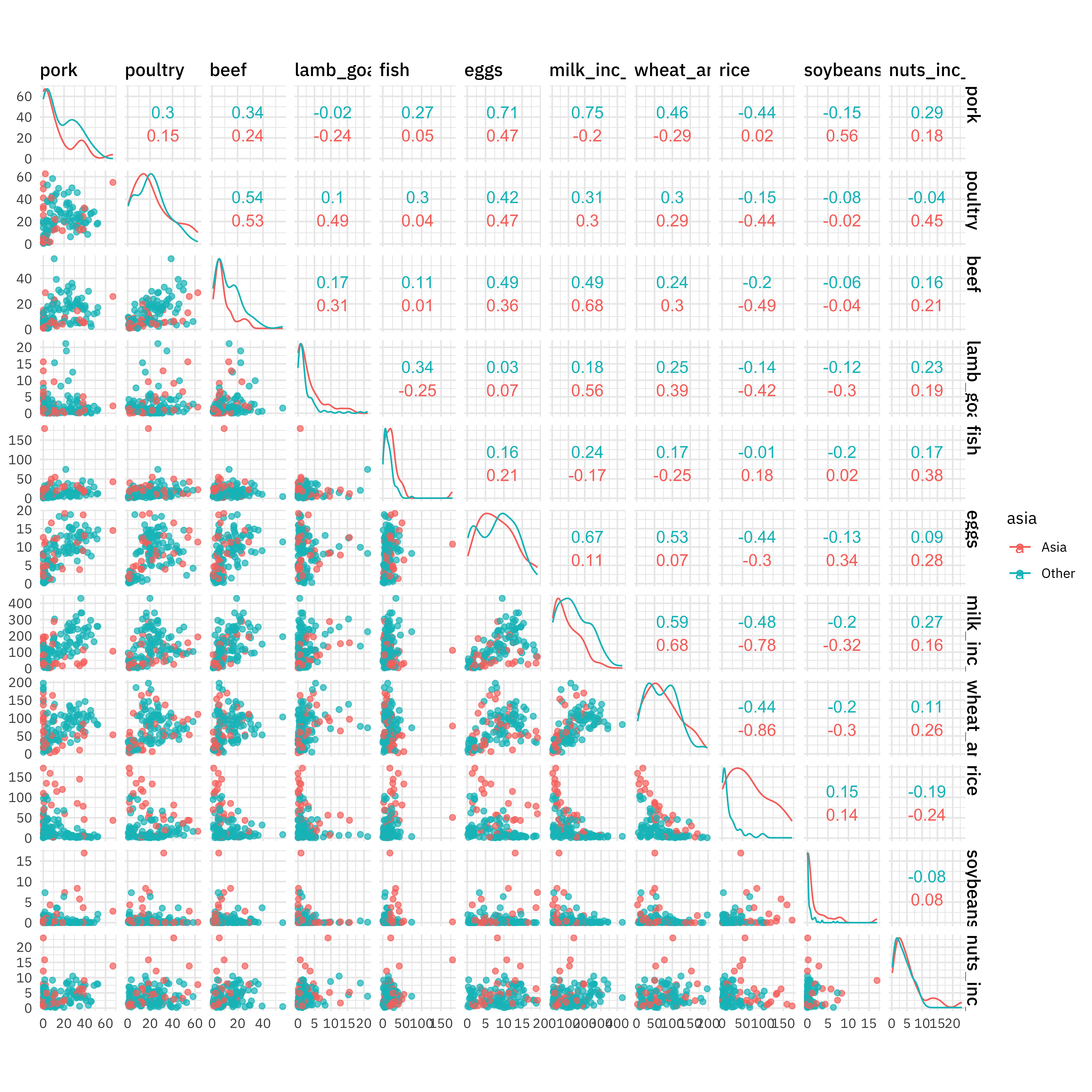
Notice how important rice is! Also see how the relationships between different food categories is different for Asian and non-Asian countries; a tree-based model like a random forest is good as learning interactions like this.

Tune hyperparameters

Now it’s time to tune the hyperparameters for a random forest model. First, let’s create a set of bootstrap resamples to use for tuning, and then let’s create a model specification for a random forest where we will tune mtry (the number of predictors to sample at each split) and min_n (the number of observations needed to keep splitting nodes). There are hyperparameters that can’t be learned from data when training the model.

library(tidymodels)

set.seed(1234)
food_boot <- bootstraps(food, times = 30)
food_boot

## # Bootstrap sampling
## # A tibble: 30 x 2
##    splits           id
##    <list>           <chr>
##  1 <split [130/48]> Bootstrap01
##  2 <split [130/49]> Bootstrap02
##  3 <split [130/49]> Bootstrap03
##  4 <split [130/51]> Bootstrap04
##  5 <split [130/47]> Bootstrap05
##  6 <split [130/51]> Bootstrap06
##  7 <split [130/57]> Bootstrap07
##  8 <split [130/51]> Bootstrap08
##  9 <split [130/44]> Bootstrap09
## 10 <split [130/53]> Bootstrap10
## # … with 20 more rows

rf_spec <- rand_forest(
  mode = "classification",
  mtry = tune(),
  trees = 1000,
  min_n = tune()
) %>%
  set_engine("ranger")

rf_spec

## Random Forest Model Specification (classification)
##
## Main Arguments:
##   mtry = tune()
##   trees = 1000
##   min_n = tune()
##
## Computational engine: ranger

We can’t learn the right values when training a single model, but we can train a whole bunch of models and see which ones turn out best. We can use parallel processing to make this go faster, since the different parts of the grid are independent.

doParallel::registerDoParallel()

rf_grid <- tune_grid(
  asia ~ .,
  model = rf_spec,
  resamples = food_boot
)

rf_grid

## # Bootstrap sampling
## # A tibble: 30 x 4
##    splits           id          .metrics          .notes
##    <list>           <chr>       <list>            <list>
##  1 <split [130/48]> Bootstrap01 <tibble [20 × 5]> <tibble [0 × 1]>
##  2 <split [130/49]> Bootstrap02 <tibble [20 × 5]> <tibble [0 × 1]>
##  3 <split [130/49]> Bootstrap03 <tibble [20 × 5]> <tibble [0 × 1]>
##  4 <split [130/51]> Bootstrap04 <tibble [20 × 5]> <tibble [0 × 1]>
##  5 <split [130/47]> Bootstrap05 <tibble [20 × 5]> <tibble [0 × 1]>
##  6 <split [130/51]> Bootstrap06 <tibble [20 × 5]> <tibble [0 × 1]>
##  7 <split [130/57]> Bootstrap07 <tibble [20 × 5]> <tibble [0 × 1]>
##  8 <split [130/51]> Bootstrap08 <tibble [20 × 5]> <tibble [0 × 1]>
##  9 <split [130/44]> Bootstrap09 <tibble [20 × 5]> <tibble [0 × 1]>
## 10 <split [130/53]> Bootstrap10 <tibble [20 × 5]> <tibble [0 × 1]>
## # … with 20 more rows

Once we have our tuning results, we can check them out.

rf_grid %>%
  collect_metrics()

## # A tibble: 20 x 7
##     mtry min_n .metric  .estimator  mean     n std_err
##    <int> <int> <chr>    <chr>      <dbl> <int>   <dbl>
##  1     2     4 accuracy binary     0.836    30 0.00801
##  2     2     4 roc_auc  binary     0.841    30 0.00942
##  3     2    12 accuracy binary     0.826    30 0.00779
##  4     2    12 roc_auc  binary     0.837    30 0.00902
##  5     4    33 accuracy binary     0.817    30 0.00895
##  6     4    33 roc_auc  binary     0.820    30 0.0105
##  7     4    37 accuracy binary     0.813    30 0.00851
##  8     4    37 roc_auc  binary     0.818    30 0.0102
##  9     5    31 accuracy binary     0.817    30 0.00875
## 10     5    31 roc_auc  binary     0.819    30 0.0103
## 11     6     9 accuracy binary     0.826    30 0.00954
## 12     6     9 roc_auc  binary     0.832    30 0.00956
## 13     7    21 accuracy binary     0.814    30 0.00926
## 14     7    21 roc_auc  binary     0.823    30 0.0103
## 15     8    18 accuracy binary     0.822    30 0.00887
## 16     8    18 roc_auc  binary     0.823    30 0.0104
## 17     9    26 accuracy binary     0.815    30 0.00992
## 18     9    26 roc_auc  binary     0.822    30 0.0109
## 19    11    15 accuracy binary     0.812    30 0.0114
## 20    11    15 roc_auc  binary     0.822    30 0.0102

And we can see which models performed the best, in terms of some given metric.

rf_grid %>%
  show_best("roc_auc")

## # A tibble: 5 x 7
##    mtry min_n .metric .estimator  mean     n std_err
##   <int> <int> <chr>   <chr>      <dbl> <int>   <dbl>
## 1     2     4 roc_auc binary     0.841    30 0.00942
## 2     2    12 roc_auc binary     0.837    30 0.00902
## 3     6     9 roc_auc binary     0.832    30 0.00956
## 4     8    18 roc_auc binary     0.823    30 0.0104
## 5     7    21 roc_auc binary     0.823    30 0.0103

If you would like to specific the grid for tuning yourself, check out the dials package!