#TidyTuesday hotel bookings and recipes
By Julia Silge in rstats tidymodels
February 11, 2020
Last week I published
my first screencast showing how to use the tidymodels framework for machine learning and modeling in R. Today, I’m using this week’s
#TidyTuesday dataset on hotel bookings to show how to use one of the tidymodels packages
recipes with some simple models!
Here is the code I used in the video, for those who prefer reading instead of or in addition to video.
Explore the data
Our modeling goal here is to predict which hotel stays include children (vs. do not include children or babies) based on the other characteristics in this dataset such as which hotel the guests stay at, how much they pay, etc. The paper that this data comes from points out that the distribution of many of these variables (such as number of adults/children, room type, meals bought, country, and so forth) is different for canceled vs. not canceled hotel bookings. This is mostly because more information is gathered when guests check in; the biggest contributor to these differences is not that people who cancel are different from people who do not.
To build our models, let’s filter to only the bookings that did not cancel and build a model to predict which hotel stays include children and which do not.
library(tidyverse)

hotels <- readr::read_csv("https://raw.githubusercontent.com/rfordatascience/tidytuesday/master/data/2020/2020-02-11/hotels.csv")


hotel_stays <- hotels %>%
  filter(is_canceled == 0) %>%
  mutate(
    children = case_when(
      children + babies > 0 ~ "children",
      TRUE ~ "none"
    ),
    required_car_parking_spaces = case_when(
      required_car_parking_spaces > 0 ~ "parking",
      TRUE ~ "none"
    )
  ) %>%
  select(-is_canceled, -reservation_status, -babies)

hotel_stays
## # A tibble: 75,166 x 29
##    hotel lead_time arrival_date_ye… arrival_date_mo… arrival_date_we…
##    <chr>     <dbl>            <dbl> <chr>                       <dbl>
##  1 Reso…       342             2015 July                           27
##  2 Reso…       737             2015 July                           27
##  3 Reso…         7             2015 July                           27
##  4 Reso…        13             2015 July                           27
##  5 Reso…        14             2015 July                           27
##  6 Reso…        14             2015 July                           27
##  7 Reso…         0             2015 July                           27
##  8 Reso…         9             2015 July                           27
##  9 Reso…        35             2015 July                           27
## 10 Reso…        68             2015 July                           27
## # … with 75,156 more rows, and 24 more variables:
## #   arrival_date_day_of_month <dbl>, stays_in_weekend_nights <dbl>,
## #   stays_in_week_nights <dbl>, adults <dbl>, children <chr>, meal <chr>,
## #   country <chr>, market_segment <chr>, distribution_channel <chr>,
## #   is_repeated_guest <dbl>, previous_cancellations <dbl>,
## #   previous_bookings_not_canceled <dbl>, reserved_room_type <chr>,
## #   assigned_room_type <chr>, booking_changes <dbl>, deposit_type <chr>,
## #   agent <chr>, company <chr>, days_in_waiting_list <dbl>,
## #   customer_type <chr>, adr <dbl>, required_car_parking_spaces <chr>,
## #   total_of_special_requests <dbl>, reservation_status_date <date>
hotel_stays %>%
  count(children)
## # A tibble: 2 x 2
##   children     n
##   <chr>    <int>
## 1 children  6073
## 2 none     69093
There are more than 10x more hotel stays without children than with.
When I have a new dataset like this one, I often use the skimr package to get an overview of the dataset’s characteristics. The numeric variables here have different very different values and distributions (big vs. small).
library(skimr)

skim(hotel_stays)
## ── Data Summary ────────────────────────
##                            Values
## Name                       hotel_stays
## Number of rows             75166
## Number of columns          29
## _______________________
## Column type frequency:
##   character                14
##   Date                     1
##   numeric                  14
## ________________________
## Group variables            None
##
## ── Variable type: character ────────────────────────────────────────────────────
##    skim_variable               n_missing complete_rate   min   max empty
##  1 hotel                               0             1    10    12     0
##  2 arrival_date_month                  0             1     3     9     0
##  3 children                            0             1     4     8     0
##  4 meal                                0             1     2     9     0
##  5 country                             0             1     2     4     0
##  6 market_segment                      0             1     6    13     0
##  7 distribution_channel                0             1     3     9     0
##  8 reserved_room_type                  0             1     1     1     0
##  9 assigned_room_type                  0             1     1     1     0
## 10 deposit_type                        0             1    10    10     0
## 11 agent                               0             1     1     4     0
## 12 company                             0             1     1     4     0
## 13 customer_type                       0             1     5    15     0
## 14 required_car_parking_spaces         0             1     4     7     0
##    n_unique whitespace
##  1        2          0
##  2       12          0
##  3        2          0
##  4        5          0
##  5      166          0
##  6        7          0
##  7        5          0
##  8        9          0
##  9       10          0
## 10        3          0
## 11      315          0
## 12      332          0
## 13        4          0
## 14        2          0
##
## ── Variable type: Date ─────────────────────────────────────────────────────────
##   skim_variable           n_missing complete_rate min        max
## 1 reservation_status_date         0             1 2015-07-01 2017-09-14
##   median     n_unique
## 1 2016-09-01      805
##
## ── Variable type: numeric ──────────────────────────────────────────────────────
##    skim_variable                  n_missing complete_rate      mean     sd
##  1 lead_time                              0             1   80.0    91.1
##  2 arrival_date_year                      0             1 2016.      0.703
##  3 arrival_date_week_number               0             1   27.1    13.9
##  4 arrival_date_day_of_month              0             1   15.8     8.78
##  5 stays_in_weekend_nights                0             1    0.929   0.993
##  6 stays_in_week_nights                   0             1    2.46    1.92
##  7 adults                                 0             1    1.83    0.510
##  8 is_repeated_guest                      0             1    0.0433  0.204
##  9 previous_cancellations                 0             1    0.0158  0.272
## 10 previous_bookings_not_canceled         0             1    0.203   1.81
## 11 booking_changes                        0             1    0.293   0.736
## 12 days_in_waiting_list                   0             1    1.59   14.8
## 13 adr                                    0             1  100.     49.2
## 14 total_of_special_requests              0             1    0.714   0.834
##         p0    p25    p50   p75  p100 hist
##  1    0       9     45     124   737 ▇▂▁▁▁
##  2 2015    2016   2016    2017  2017 ▃▁▇▁▆
##  3    1      16     28      38    53 ▆▇▇▇▆
##  4    1       8     16      23    31 ▇▇▇▇▆
##  5    0       0      1       2    19 ▇▁▁▁▁
##  6    0       1      2       3    50 ▇▁▁▁▁
##  7    0       2      2       2     4 ▁▂▇▁▁
##  8    0       0      0       0     1 ▇▁▁▁▁
##  9    0       0      0       0    13 ▇▁▁▁▁
## 10    0       0      0       0    72 ▇▁▁▁▁
## 11    0       0      0       0    21 ▇▁▁▁▁
## 12    0       0      0       0   379 ▇▁▁▁▁
## 13   -6.38   67.5   92.5   125   510 ▇▆▁▁▁
## 14    0       0      1       1     5 ▇▁▁▁▁
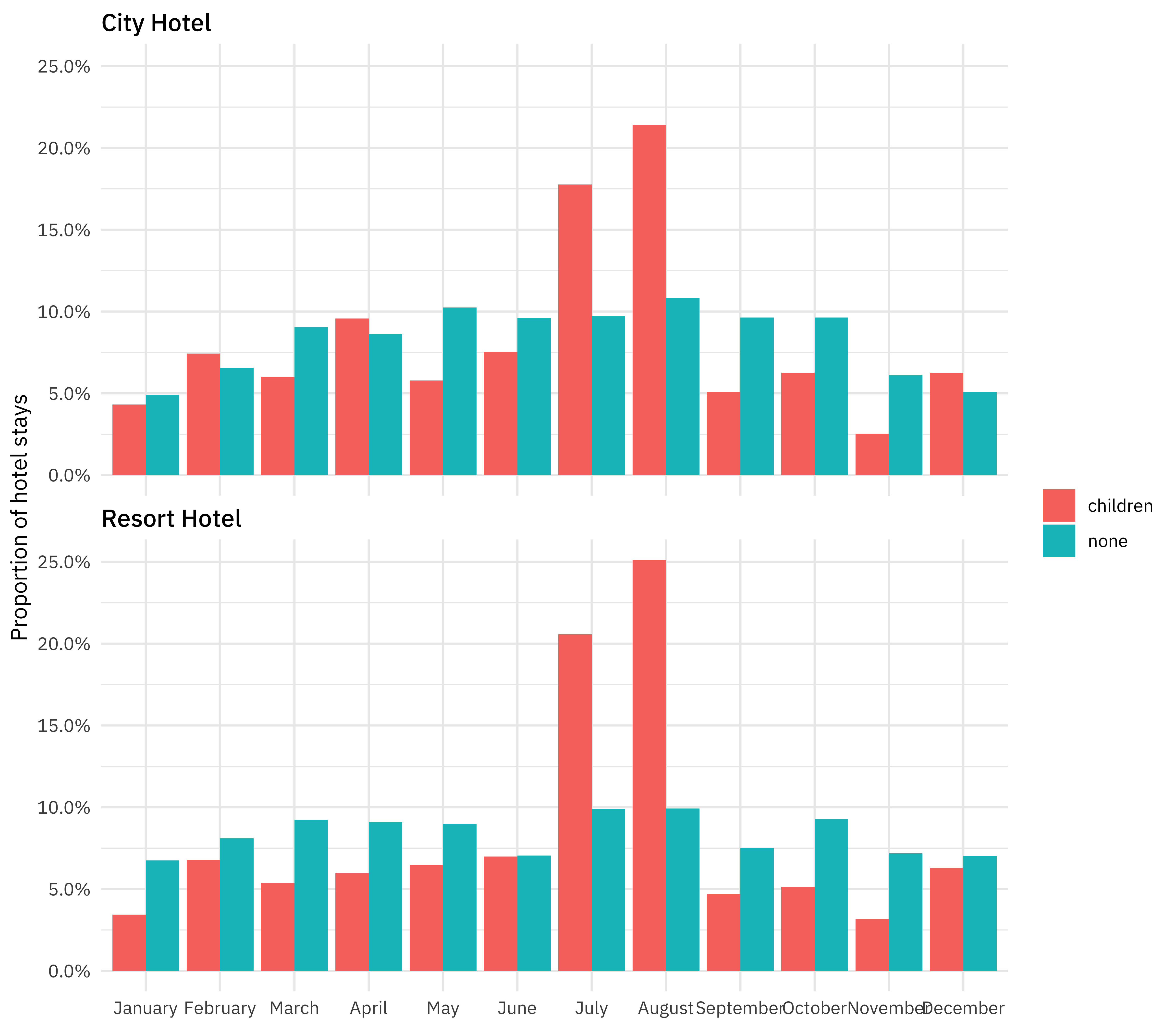
How do the hotel stays of guests with/without children vary throughout the year? Is this different in the city and the resort hotel?
hotel_stays %>%
  mutate(arrival_date_month = factor(arrival_date_month,
    levels = month.name
  )) %>%
  count(hotel, arrival_date_month, children) %>%
  group_by(hotel, children) %>%
  mutate(proportion = n / sum(n)) %>%
  ggplot(aes(arrival_date_month, proportion, fill = children)) +
  geom_col(position = "dodge") +
  scale_y_continuous(labels = scales::percent_format()) +
  facet_wrap(~hotel, nrow = 2) +
  labs(
    x = NULL,
    y = "Proportion of hotel stays",
    fill = NULL
  )
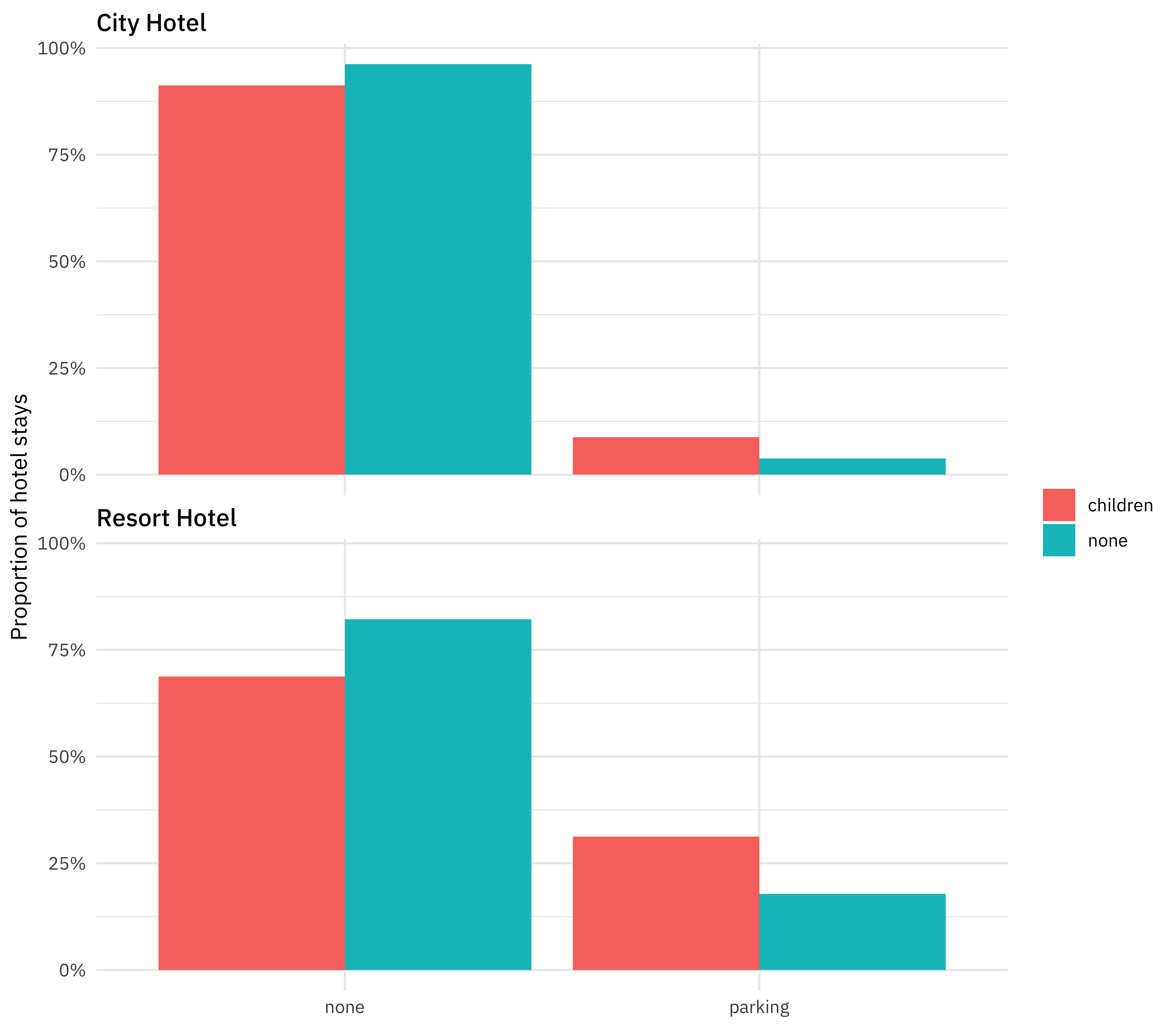
Are hotel guests with children more likely to require a parking space?
hotel_stays %>%
  count(hotel, required_car_parking_spaces, children) %>%
  group_by(hotel, children) %>%
  mutate(proportion = n / sum(n)) %>%
  ggplot(aes(required_car_parking_spaces, proportion, fill = children)) +
  geom_col(position = "dodge") +
  scale_y_continuous(labels = scales::percent_format()) +
  facet_wrap(~hotel, nrow = 2) +
  labs(
    x = NULL,
    y = "Proportion of hotel stays",
    fill = NULL
  )
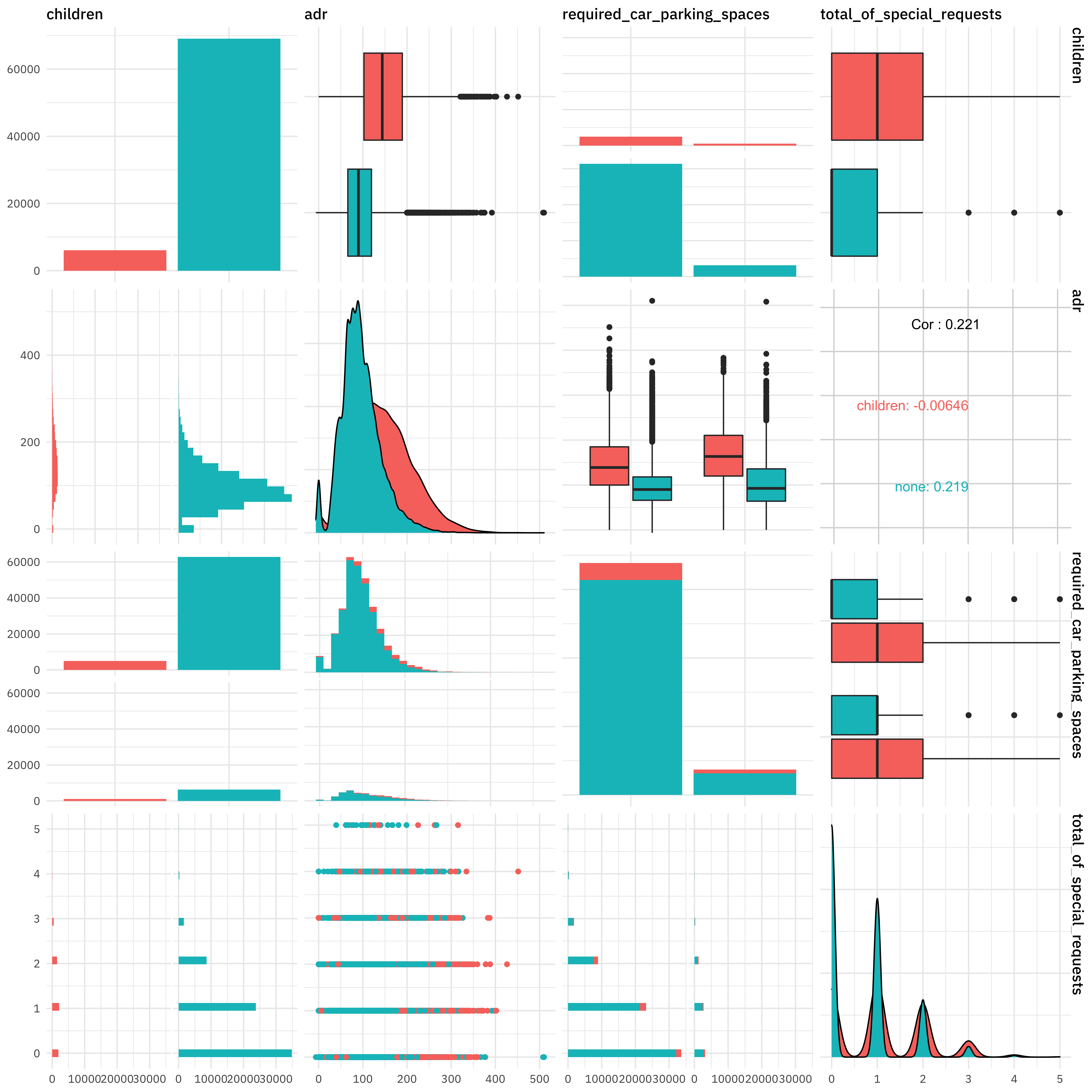
There are many more relationships like this we can explore. In many situations I like to use the ggpairs() function to get a high-level view of how variables are related to each other.
library(GGally)

hotel_stays %>%
  select(
    children, adr,
    required_car_parking_spaces,
    total_of_special_requests
  ) %>%
  ggpairs(mapping = aes(color = children))
To see more examples of EDA for this dataset, you can see the great work that folks share on Twitter! ✨
Build models with recipes
The next step for us is to create a dataset for modeling. Let’s include a set of columns we are interested in, and convert all the character columns to factors, for the modeling functions coming later.
hotels_df <- hotel_stays %>%
  select(
    children, hotel, arrival_date_month, meal, adr, adults,
    required_car_parking_spaces, total_of_special_requests,
    stays_in_week_nights, stays_in_weekend_nights
  ) %>%
  mutate_if(is.character, factor)
Now it is time for
tidymodels! The first few lines here may
look familiar from last time; we split the data into training and testing sets using initial_split(). Next, we use a recipe() to build a set of steps for data preprocessing and feature engineering.
- First, we must tell the
recipe()what our model is going to be (using a formula here) and what our training data is. - We then downsample the data, since there are about 10x more hotel stays without children than with. If we don’t do this, our model will learn very effectively about how to predict the negative case. 😞
- We then convert the factor columns into (one or more) numeric binary (0 and 1) variables for the levels of the training data.
- Next, we remove any numeric variables that have zero variance.
- As a last step, we normalize (center and scale) the numeric variables. We need to do this because some of them are on very different scales from each other and the model we want to train is sensitive to this.
- Finally, we
prep()therecipe(). This means we actually do something with the steps and our training data; we estimate the required parameters fromhotel_trainto implement these steps so this whole sequence can be applied later to another dataset.
We then can do exactly that, and apply these transformations to the testing data; the function for this is bake(). We won’t touch the testing set again until the very end.
library(tidymodels)

set.seed(1234)
hotel_split <- initial_split(hotels_df)

hotel_train <- training(hotel_split)
hotel_test <- testing(hotel_split)

hotel_rec <- recipe(children ~ ., data = hotel_train) %>%
  step_downsample(children) %>%
  step_dummy(all_nominal(), -all_outcomes()) %>%
  step_zv(all_numeric()) %>%
  step_normalize(all_numeric()) %>%
  prep()

hotel_rec
## Data Recipe
##
## Inputs:
##
##       role #variables
##    outcome          1
##  predictor          9
##
## Training data contained 56375 data points and no missing data.
##
## Operations:
##
## Down-sampling based on children [trained]
## Dummy variables from hotel, arrival_date_month, ... [trained]
## Zero variance filter removed no terms [trained]
## Centering and scaling for adr, adults, ... [trained]
test_proc <- bake(hotel_rec, new_data = hotel_test)
Now it’s time to specify and then fit our models. First we specify and fit a nearest neighbors classification model, and then a decision tree classification model. Check out what data we are training these models on: juice(hotel_rec). The recipe hotel_rec contains all our transformations for data preprocessing and feature engineering, as well as the data these transformations were estimated from. When we juice() the recipe, we squeeze that training data back out, transformed in the ways we specified including the downsampling. The object juice(hotel_rec) is a dataframe with 9,176 rows while the our original training data hotel_train has 56,375 rows.
knn_spec <- nearest_neighbor() %>%
  set_engine("kknn") %>%
  set_mode("classification")

knn_fit <- knn_spec %>%
  fit(children ~ ., data = juice(hotel_rec))

knn_fit
## parsnip model object
##
## Fit time:  1.4s
##
## Call:
## kknn::train.kknn(formula = formula, data = data, ks = 5)
##
## Type of response variable: nominal
## Minimal misclassification: 0.2518527
## Best kernel: optimal
## Best k: 5
tree_spec <- decision_tree() %>%
  set_engine("rpart") %>%
  set_mode("classification")

tree_fit <- tree_spec %>%
  fit(children ~ ., data = juice(hotel_rec))

tree_fit
## parsnip model object
##
## Fit time:  287ms
## n= 9176
##
## node), split, n, loss, yval, (yprob)
##       * denotes terminal node
##
##  1) root 9176 4588 children (0.5000000 0.5000000)
##    2) adr>=-0.03405154 4059 1092 children (0.7309682 0.2690318) *
##    3) adr< -0.03405154 5117 1621 none (0.3167872 0.6832128)
##      6) total_of_special_requests>=0.647359 944  416 children (0.5593220 0.4406780) *
##      7) total_of_special_requests< 0.647359 4173 1093 none (0.2619219 0.7380781)
##       14) adults< -2.852103 80    9 children (0.8875000 0.1125000) *
##       15) adults>=-2.852103 4093 1022 none (0.2496946 0.7503054) *
We trained these models on the downsampled training data; we have not touched the testing data.
Evaluate models
To evaluate these models, let’s build a validation set. We can build a set of Monte Carlo splits from the downsampled training data (juice(hotel_rec)) and use this set of resamples to estimate the performance of our two models using the fit_resamples() function. This function does not do any tuning of the model parameters; in fact, it does not even keep the models it trains. This function is used for computing performance metrics across some set of resamples like our validation splits. It will fit a model such as knn_spec to each resample and evaluate on the heldout bit from each resample, and then we can collect_metrics() from the result.
set.seed(1234)
validation_splits <- mc_cv(juice(hotel_rec), prop = 0.9, strata = children)
validation_splits
## # Monte Carlo cross-validation (0.9/0.1) with 25 resamples  using stratification
## # A tibble: 25 x 2
##    splits             id
##    <named list>       <chr>
##  1 <split [8.3K/916]> Resample01
##  2 <split [8.3K/916]> Resample02
##  3 <split [8.3K/916]> Resample03
##  4 <split [8.3K/916]> Resample04
##  5 <split [8.3K/916]> Resample05
##  6 <split [8.3K/916]> Resample06
##  7 <split [8.3K/916]> Resample07
##  8 <split [8.3K/916]> Resample08
##  9 <split [8.3K/916]> Resample09
## 10 <split [8.3K/916]> Resample10
## # … with 15 more rows
knn_res <- fit_resamples(
  children ~ .,
  knn_spec,
  validation_splits,
  control = control_resamples(save_pred = TRUE)
)

knn_res %>%
  collect_metrics()
## # A tibble: 2 x 5
##   .metric  .estimator  mean     n std_err
##   <chr>    <chr>      <dbl> <int>   <dbl>
## 1 accuracy binary     0.74     25 0.00272
## 2 roc_auc  binary     0.804    25 0.00219
tree_res <- fit_resamples(
  children ~ .,
  tree_spec,
  validation_splits,
  control = control_resamples(save_pred = TRUE)
)

tree_res %>%
  collect_metrics()
## # A tibble: 2 x 5
##   .metric  .estimator  mean     n std_err
##   <chr>    <chr>      <dbl> <int>   <dbl>
## 1 accuracy binary     0.722    25 0.00248
## 2 roc_auc  binary     0.741    25 0.00230
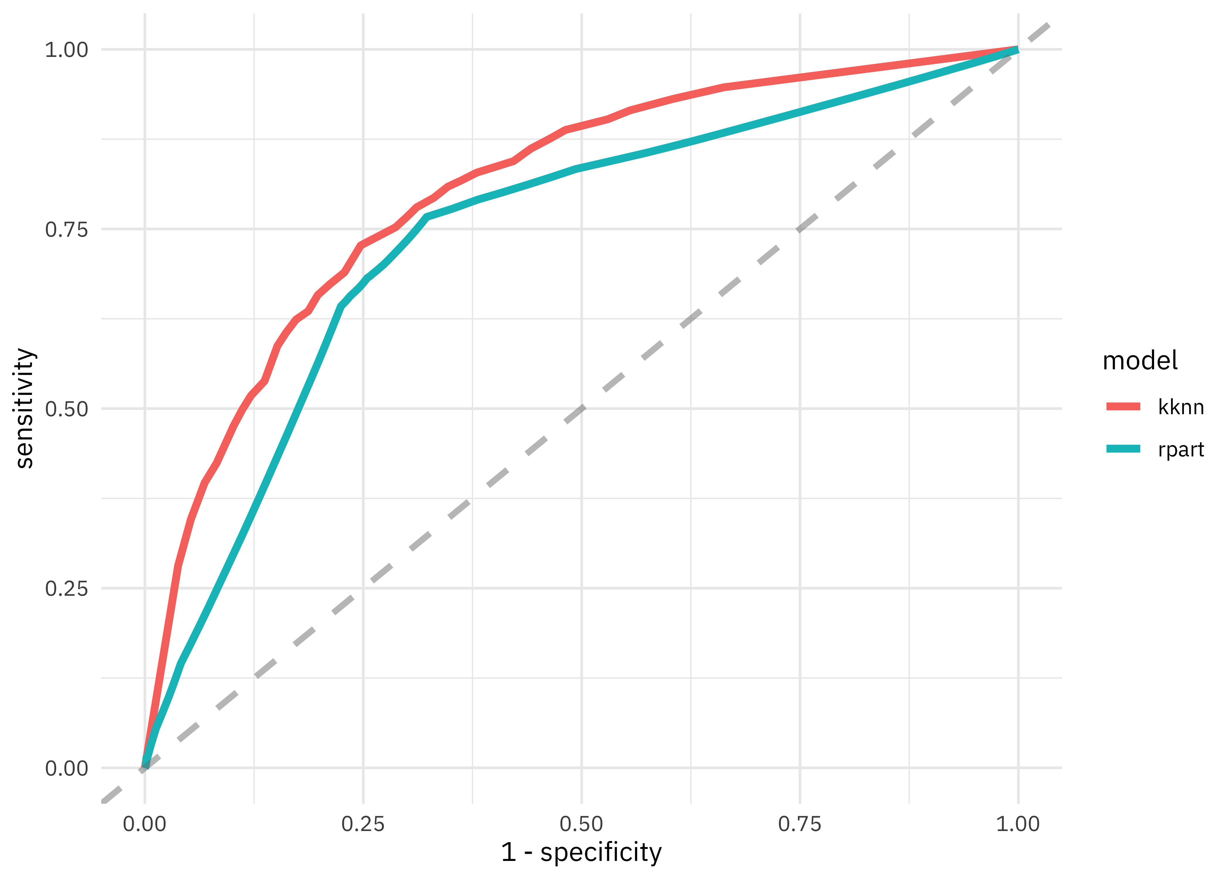
This validation set gives us a better estimate of how our models are doing than predicting the whole training set at once. The nearest neighbor model performs somewhat better than the decision tree. Let’s visualize these results.
knn_res %>%
  unnest(.predictions) %>%
  mutate(model = "kknn") %>%
  bind_rows(tree_res %>%
    unnest(.predictions) %>%
    mutate(model = "rpart")) %>%
  group_by(model) %>%
  roc_curve(children, .pred_children) %>%
  ggplot(aes(x = 1 - specificity, y = sensitivity, color = model)) +
  geom_line(size = 1.5) +
  geom_abline(
    lty = 2, alpha = 0.5,
    color = "gray50",
    size = 1.2
  )
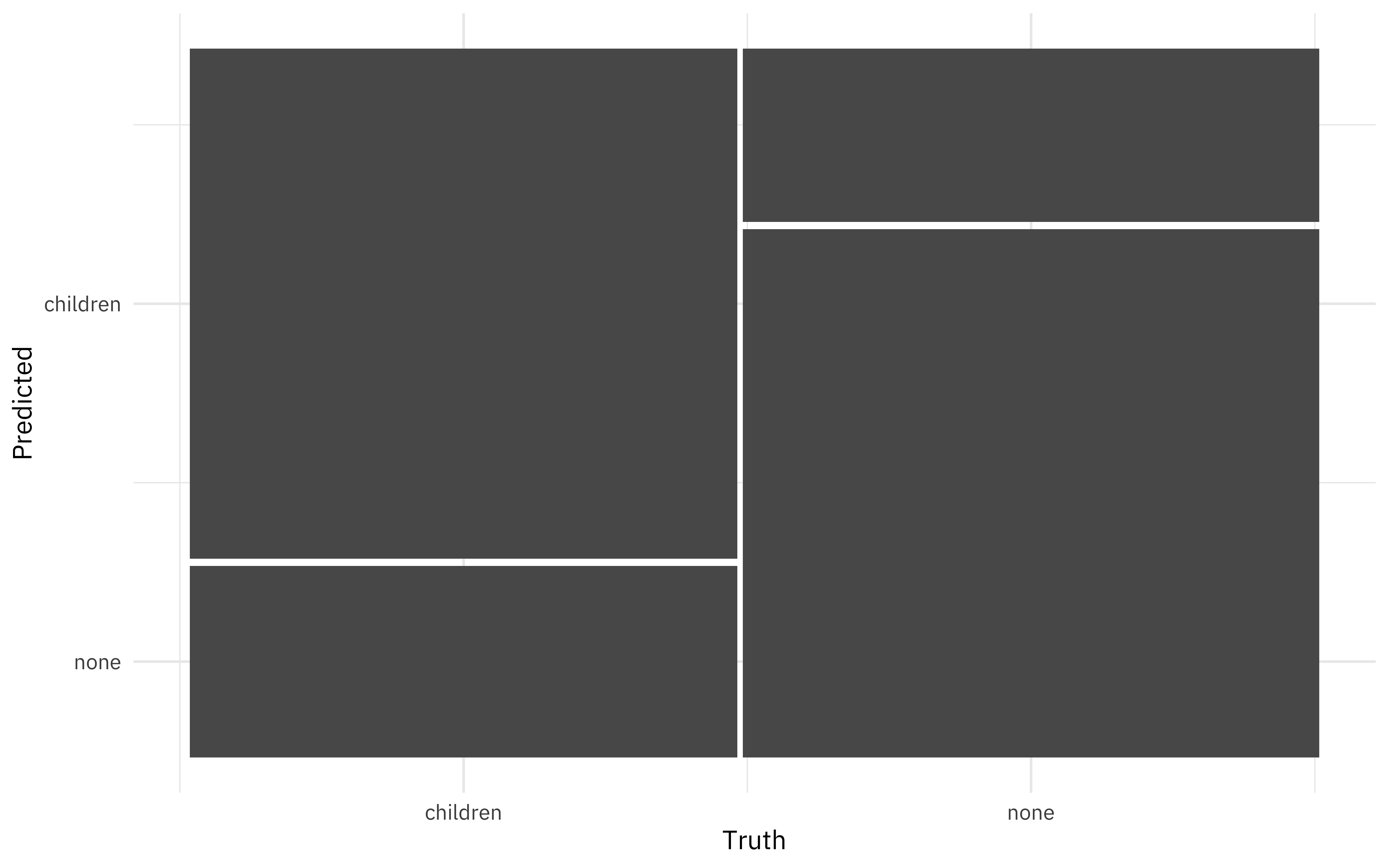
We can also create a confusion matrix.
knn_conf <- knn_res %>%
  unnest(.predictions) %>%
  conf_mat(children, .pred_class)

knn_conf
##           Truth
## Prediction children none
##   children     8325 2829
##   none         3125 8621
knn_conf %>%
  autoplot()
FINALLY, let’s check in with our transformed testing data and see how we can expect this model to perform on new data.
knn_fit %>%
  predict(new_data = test_proc, type = "prob") %>%
  mutate(truth = hotel_test$children) %>%
  roc_auc(truth, .pred_children)
## # A tibble: 1 x 3
##   .metric .estimator .estimate
##   <chr>   <chr>          <dbl>
## 1 roc_auc binary         0.795
Notice that this AUC value is about the same as from our validation splits.
Summary
Let me know if you have questions or feedback about using recipes with tidymodels and how to get started. I am glad to be using these #TidyTuesday datasets for predictive modeling!
- Posted on:
- February 11, 2020
- Length:
- 12 minute read, 2404 words
- Categories:
- rstats tidymodels
- Tags:
- rstats tidymodels