Preprocessing and resampling using #TidyTuesday college data

I’ve been publishing screencasts demonstrating how to use the tidymodels framework, from first getting started to how to tune machine learning models. Today, I’m using this week’s #TidyTuesday dataset on college tuition and diversity at US colleges to show some data preprocessing steps and how to use resampling!

Here is the code I used in the video, for those who prefer reading instead of or in addition to video.

Explore the data

Our modeling goal here is to predict which US colleges have higher proportions of minority students based on college data such as tuition from the #TidyTuesday dataset. There are several related datasets this week, and this modeling analysis uses two of them.

library(tidyverse)

tuition_cost <- readr::read_csv("https://raw.githubusercontent.com/rfordatascience/tidytuesday/master/data/2020/2020-03-10/tuition_cost.csv")

diversity_raw <- readr::read_csv("https://raw.githubusercontent.com/rfordatascience/tidytuesday/master/data/2020/2020-03-10/diversity_school.csv") %>%
  filter(category == "Total Minority") %>%
  mutate(TotalMinority = enrollment / total_enrollment)

What is the distribution of total minority student population?

diversity_school <- diversity_raw %>%
  filter(category == "Total Minority") %>%
  mutate(TotalMinority = enrollment / total_enrollment)

diversity_school %>%
  ggplot(aes(TotalMinority)) +
  geom_histogram(alpha = 0.7, fill = "midnightblue") +
  scale_x_continuous(labels = scales::percent_format()) +
  labs(x = "% of student population who identifies as any minority")

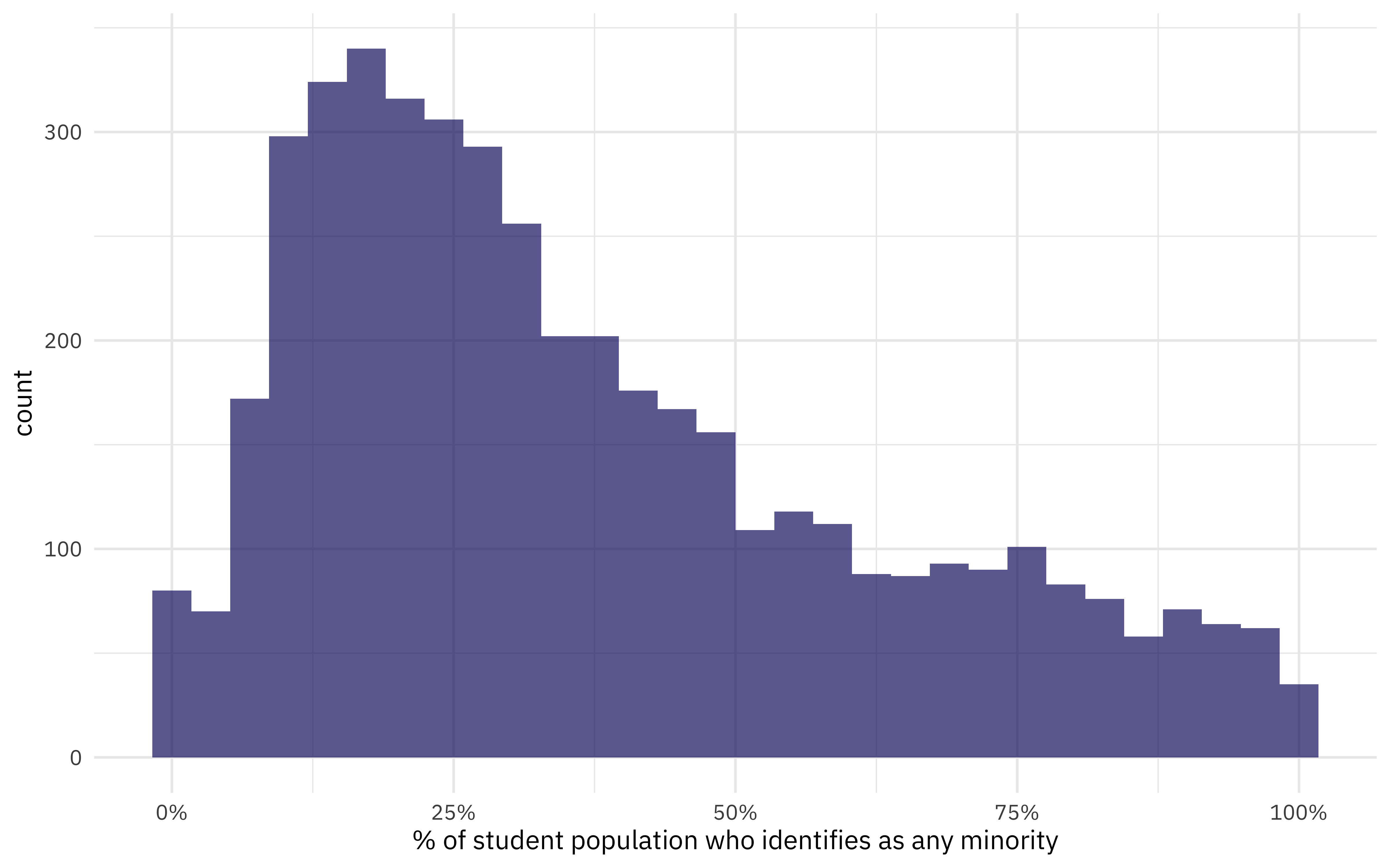
The median proportion of minority students for this dataset is 30%.

Let’s build a dataset for modeling, joining the two dataframes we have. Let’s also move from individual states in the US to US regions, as found in state.region.

university_df <- diversity_school %>%
  filter(category == "Total Minority") %>%
  mutate(TotalMinority = enrollment / total_enrollment) %>%
  transmute(
    diversity = case_when(
      TotalMinority > 0.3 ~ "high",
      TRUE ~ "low"
    ),
    name, state,
    total_enrollment
  ) %>%
  inner_join(tuition_cost %>%
    select(
      name, type, degree_length,
      in_state_tuition:out_of_state_total
    )) %>%
  left_join(tibble(state = state.name, region = state.region)) %>%
  select(-state, -name) %>%
  mutate_if(is.character, factor)

skimr::skim(university_df)

## ── Data Summary ────────────────────────
##                            Values
## Name                       university_df
## Number of rows             2159
## Number of columns          9
## _______________________
## Column type frequency:
##   factor                   4
##   numeric                  5
## ________________________
## Group variables            None
##
## ── Variable type: factor ───────────────────────────────────────────────────────
##   skim_variable n_missing complete_rate ordered n_unique
## 1 diversity             0             1 FALSE          2
## 2 type                  0             1 FALSE          3
## 3 degree_length         0             1 FALSE          2
## 4 region                0             1 FALSE          4
##   top_counts
## 1 low: 1241, hig: 918
## 2 Pub: 1145, Pri: 955, For: 59
## 3 4 Y: 1296, 2 Y: 863
## 4 Sou: 774, Nor: 543, Nor: 443, Wes: 399
##
## ── Variable type: numeric ──────────────────────────────────────────────────────
##   skim_variable        n_missing complete_rate   mean     sd    p0   p25   p50
## 1 total_enrollment             0             1  6184.  8264.    15  1352  3133
## 2 in_state_tuition             0             1 17044. 15461.   480  4695 10161
## 3 in_state_total               0             1 23545. 19782.   962  5552 17749
## 4 out_of_state_tuition         0             1 20798. 13725.   480  9298 17045
## 5 out_of_state_total           0             1 27299. 18221.  1376 11018 23036
##      p75  p100 hist
## 1  7644. 81459 ▇▁▁▁▁
## 2 28780  59985 ▇▂▂▁▁
## 3 38519  75003 ▇▅▂▂▁
## 4 29865  59985 ▇▆▅▂▁
## 5 40154  75003 ▇▅▅▂▁

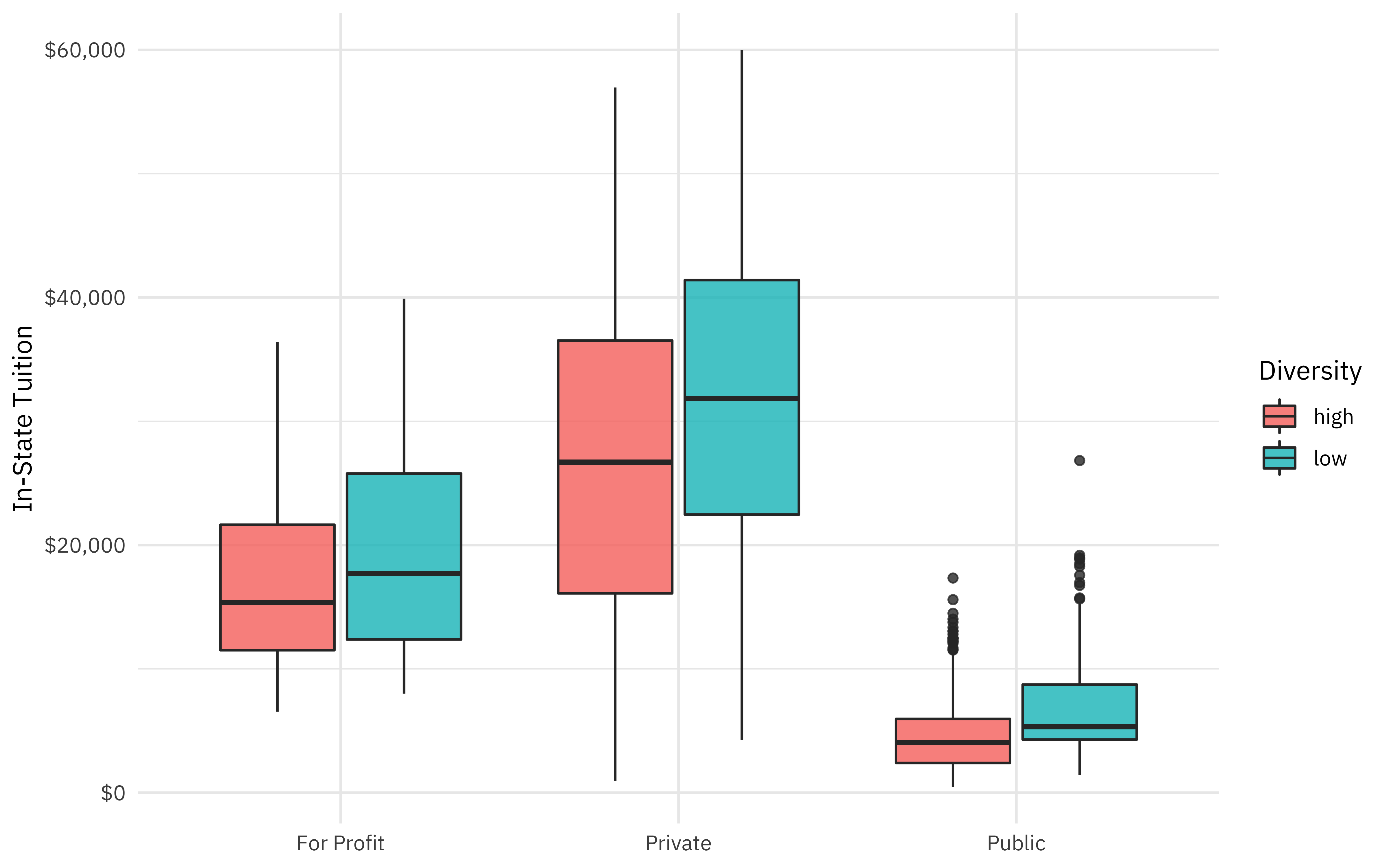
How are some of these quantities related to the proportion of minority students at a college?

university_df %>%
  ggplot(aes(type, in_state_tuition, fill = diversity)) +
  geom_boxplot(alpha = 0.8) +
  scale_y_continuous(labels = scales::dollar_format()) +
  labs(x = NULL, y = "In-State Tuition", fill = "Diversity")

Build models with recipes

Now it is time for modeling! First, we split our data into training and testing sets. Then, we build a recipe for data preprocessing.

• First, we must tell the recipe() what our model is going to be (using a formula here) and what our training data is.
• We then filter out variables that are too correlated with each other. We had several different ways of measuring the tuition in our dataset that are correlated with each other, and this step shows how to handle a situation like that.
• We then convert the factor columns into (one or more) numeric binary (0 and 1) variables for the levels of the training data.
• Next, we remove any numeric variables that have zero variance.
• As a last step, we normalize (center and scale) the numeric variables. We need to do this because some of them are on very different scales from each other and a model we want to train is sensitive to this.
• Finally, we prep() the recipe(). This means we actually do something with the steps and our training data; we estimate the required parameters from uni_train to implement these steps so this whole sequence can be applied later to another dataset.

library(tidymodels)

set.seed(1234)
uni_split <- initial_split(university_df, strata = diversity)
uni_train <- training(uni_split)
uni_test <- testing(uni_split)

uni_rec <- recipe(diversity ~ ., data = uni_train) %>%
  step_corr(all_numeric()) %>%
  step_dummy(all_nominal(), -all_outcomes()) %>%
  step_zv(all_numeric()) %>%
  step_normalize(all_numeric())

uni_prep <- uni_rec %>%
  prep()

uni_prep

## Data Recipe
##
## Inputs:
##
##       role #variables
##    outcome          1
##  predictor          8
##
## Training data contained 1620 data points and no missing data.
##
## Operations:
##
## Correlation filter removed in_state_tuition, ... [trained]
## Dummy variables from type, degree_length, region [trained]
## Zero variance filter removed no terms [trained]
## Centering and scaling for total_enrollment, ... [trained]

Now it’s time to specify and then fit our models. Here, we specify and fit three models:

• logistic regression
• k-nearest neighbor
• decision tree

Check out what data we are training these models on: juice(uni_rec). The recipe uni_rec contains all our transformations for data preprocessing and feature engineering, as well as the data these transformations were estimated from. When we juice() the recipe, we squeeze that training data back out, transformed in all the ways we specified.

uni_juiced <- juice(uni_prep)

glm_spec <- logistic_reg() %>%
  set_engine("glm")

glm_fit <- glm_spec %>%
  fit(diversity ~ ., data = uni_juiced)

glm_fit

## parsnip model object
##
## Fit time:  7ms
##
## Call:  stats::glm(formula = formula, family = stats::binomial, data = data)
##
## Coefficients:
##           (Intercept)       total_enrollment     out_of_state_total
##                0.3704                -0.4581                 0.5074
##          type_Private            type_Public  degree_length_X4.Year
##               -0.1656                 0.2058                 0.2082
##          region_South   region_North.Central            region_West
##               -0.5175                 0.3004                -0.5363
##
## Degrees of Freedom: 1619 Total (i.e. Null);  1611 Residual
## Null Deviance:	    2210
## Residual Deviance: 1859 	AIC: 1877

knn_spec <- nearest_neighbor() %>%
  set_engine("kknn") %>%
  set_mode("classification")

knn_fit <- knn_spec %>%
  fit(diversity ~ ., data = uni_juiced)

knn_fit

## parsnip model object
##
## Fit time:  54ms
##
## Call:
## kknn::train.kknn(formula = formula, data = data, ks = 5)
##
## Type of response variable: nominal
## Minimal misclassification: 0.3277778
## Best kernel: optimal
## Best k: 5

tree_spec <- decision_tree() %>%
  set_engine("rpart") %>%
  set_mode("classification")

tree_fit <- tree_spec %>%
  fit(diversity ~ ., data = uni_juiced)

tree_fit

## parsnip model object
##
## Fit time:  23ms
## n= 1620
##
## node), split, n, loss, yval, (yprob)
##       * denotes terminal node
##
##  1) root 1620 689 low (0.4253086 0.5746914)
##    2) region_North.Central< 0.5346496 1192 586 high (0.5083893 0.4916107)
##      4) out_of_state_total< -0.7087237 418 130 high (0.6889952 0.3110048) *
##      5) out_of_state_total>=-0.7087237 774 318 low (0.4108527 0.5891473)
##       10) out_of_state_total< 0.35164 362 180 low (0.4972376 0.5027624)
##         20) region_South>=0.3002561 212  86 high (0.5943396 0.4056604)
##           40) degree_length_X4.Year>=-0.2001293 172  62 high (0.6395349 0.3604651) *
##           41) degree_length_X4.Year< -0.2001293 40  16 low (0.4000000 0.6000000) *
##         21) region_South< 0.3002561 150  54 low (0.3600000 0.6400000)
##           42) region_West>=0.8128302 64  28 high (0.5625000 0.4375000) *
##           43) region_West< 0.8128302 86  18 low (0.2093023 0.7906977) *
##       11) out_of_state_total>=0.35164 412 138 low (0.3349515 0.6650485)
##         22) region_West>=0.8128302 88  38 high (0.5681818 0.4318182)
##           44) out_of_state_total>=1.547681 30   5 high (0.8333333 0.1666667) *
##           45) out_of_state_total< 1.547681 58  25 low (0.4310345 0.5689655) *
##         23) region_West< 0.8128302 324  88 low (0.2716049 0.7283951) *
##    3) region_North.Central>=0.5346496 428  83 low (0.1939252 0.8060748)
##      6) out_of_state_total< -1.19287 17   5 high (0.7058824 0.2941176) *
##      7) out_of_state_total>=-1.19287 411  71 low (0.1727494 0.8272506) *

Models! 🎉

Evaluate models with resampling

Well, we fit models, but how do we evaluate them? We can use resampling to compute performance metrics across some set of resamples, like the cross-validation splits we create here. The function fit_resamples() fits a model such as glm_spec to the analysis subset of each resample and evaluates on the heldout bit (the assessment subset) from each resample. We can use metrics = metric_set() to specify which metrics we want to compute if we don’t want to only use the default ones; here let’s check out sensitivity and specificity.

Originally in the video, I set up the resampled folds like this:

set.seed(123)
folds <- vfold_cv(uni_juiced, strata = diversity)

But some helpful folks pointed out that this can result in overly optimistic results from resampling (i.e. data leakage) because of some of the recipe steps. It’s better to resample the original training data.

set.seed(123)
folds <- vfold_cv(uni_train, strata = diversity)

After we have these folds, we can use fit_resamples() with the recipe to estimate model metrics.

set.seed(234)
glm_rs <- glm_spec %>%
  fit_resamples(
    uni_rec,
    folds,
    metrics = metric_set(roc_auc, sens, spec),
    control = control_resamples(save_pred = TRUE)
  )

set.seed(234)
knn_rs <- knn_spec %>%
  fit_resamples(
    uni_rec,
    folds,
    metrics = metric_set(roc_auc, sens, spec),
    control = control_resamples(save_pred = TRUE)
  )

set.seed(234)
tree_rs <- tree_spec %>%
  fit_resamples(
    uni_rec,
    folds,
    metrics = metric_set(roc_auc, sens, spec),
    control = control_resamples(save_pred = TRUE)
  )

What do these results look like?

tree_rs

## #  10-fold cross-validation using stratification
## # A tibble: 10 x 5
##    splits             id     .metrics         .notes           .predictions
##    <list>             <chr>  <list>           <list>           <list>
##  1 <split [1.5K/163]> Fold01 <tibble [3 × 3]> <tibble [0 × 1]> <tibble [163 × 5…
##  2 <split [1.5K/162]> Fold02 <tibble [3 × 3]> <tibble [0 × 1]> <tibble [162 × 5…
##  3 <split [1.5K/162]> Fold03 <tibble [3 × 3]> <tibble [0 × 1]> <tibble [162 × 5…
##  4 <split [1.5K/162]> Fold04 <tibble [3 × 3]> <tibble [0 × 1]> <tibble [162 × 5…
##  5 <split [1.5K/162]> Fold05 <tibble [3 × 3]> <tibble [0 × 1]> <tibble [162 × 5…
##  6 <split [1.5K/162]> Fold06 <tibble [3 × 3]> <tibble [0 × 1]> <tibble [162 × 5…
##  7 <split [1.5K/162]> Fold07 <tibble [3 × 3]> <tibble [0 × 1]> <tibble [162 × 5…
##  8 <split [1.5K/162]> Fold08 <tibble [3 × 3]> <tibble [0 × 1]> <tibble [162 × 5…
##  9 <split [1.5K/162]> Fold09 <tibble [3 × 3]> <tibble [0 × 1]> <tibble [162 × 5…
## 10 <split [1.5K/161]> Fold10 <tibble [3 × 3]> <tibble [0 × 1]> <tibble [161 × 5…

We can use collect_metrics() to see the summarized performance metrics for each set of resamples.

glm_rs %>%
  collect_metrics()

## # A tibble: 3 x 5
##   .metric .estimator  mean     n std_err
##   <chr>   <chr>      <dbl> <int>   <dbl>
## 1 roc_auc binary     0.758    10 0.00891
## 2 sens    binary     0.617    10 0.0179
## 3 spec    binary     0.737    10 0.00677

knn_rs %>%
  collect_metrics()

## # A tibble: 3 x 5
##   .metric .estimator  mean     n std_err
##   <chr>   <chr>      <dbl> <int>   <dbl>
## 1 roc_auc binary     0.728    10 0.00652
## 2 sens    binary     0.595    10 0.00978
## 3 spec    binary     0.733    10 0.0121

tree_rs %>%
  collect_metrics()

## # A tibble: 3 x 5
##   .metric .estimator  mean     n std_err
##   <chr>   <chr>      <dbl> <int>   <dbl>
## 1 roc_auc binary     0.723    10 0.00578
## 2 sens    binary     0.642    10 0.0182
## 3 spec    binary     0.745    10 0.00941

In realistic situations, we often care more about one of sensitivity or specificity than overall accuracy.

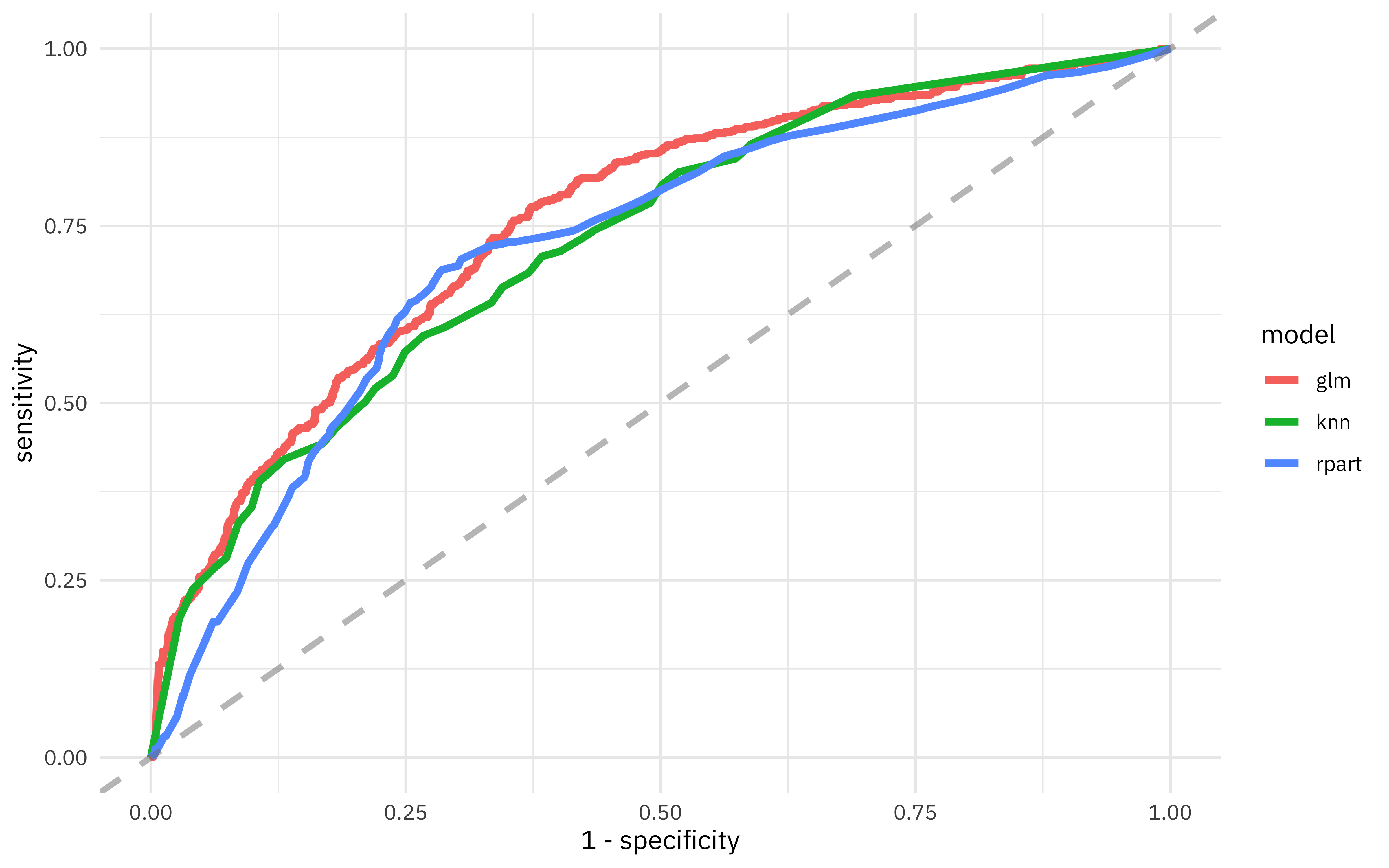
What does the ROC curve look like for these models?

glm_rs %>%
  unnest(.predictions) %>%
  mutate(model = "glm") %>%
  bind_rows(knn_rs %>%
    unnest(.predictions) %>%
    mutate(model = "knn")) %>%
  bind_rows(tree_rs %>%
    unnest(.predictions) %>%
    mutate(model = "rpart")) %>%
  group_by(model) %>%
  roc_curve(diversity, .pred_high) %>%
  ggplot(aes(x = 1 - specificity, y = sensitivity, color = model)) +
  geom_line(size = 1.5) +
  geom_abline(
    lty = 2, alpha = 0.5,
    color = "gray50",
    size = 1.2
  )

If we decide the logistic regression model is the best fit for our purposes, we can look at the parameters in detail.

glm_fit %>%
  tidy() %>%
  arrange(-estimate)

## # A tibble: 9 x 5
##   term                  estimate std.error statistic  p.value
##   <chr>                    <dbl>     <dbl>     <dbl>    <dbl>
## 1 out_of_state_total       0.507    0.0934     5.43  5.58e- 8
## 2 (Intercept)              0.370    0.0572     6.47  9.72e-11
## 3 region_North.Central     0.300    0.0825     3.64  2.72e- 4
## 4 degree_length_X4.Year    0.208    0.0863     2.41  1.58e- 2
## 5 type_Public              0.206    0.193      1.07  2.86e- 1
## 6 type_Private            -0.166    0.197     -0.838 4.02e- 1
## 7 total_enrollment        -0.458    0.0737    -6.22  5.07e-10
## 8 region_South            -0.517    0.0782    -6.62  3.64e-11
## 9 region_West             -0.536    0.0724    -7.41  1.27e-13

Larger, less expensive schools in the South and West are more likely to have higher proportions of minority students.

Finally, we can return to our test data as a last, unbiased check on how we can expect this model to perform on new data. We bake() our recipe using the testing set to apply the same preprocessing steps that we used on the training data.

glm_fit %>%
  predict(
    new_data = bake(uni_prep, uni_test),
    type = "prob"
  ) %>%
  mutate(truth = uni_test$diversity) %>%
  roc_auc(truth, .pred_high)

## # A tibble: 1 x 3
##   .metric .estimator .estimate
##   <chr>   <chr>          <dbl>
## 1 roc_auc binary         0.756

We can also explore other metrics with the test set, such as specificity.

glm_fit %>%
  predict(
    new_data = bake(uni_prep, new_data = uni_test),
    type = "class"
  ) %>%
  mutate(truth = uni_test$diversity) %>%
  spec(truth, .pred_class)

## # A tibble: 1 x 3
##   .metric .estimator .estimate
##   <chr>   <chr>          <dbl>
## 1 spec    binary         0.719

Our metrics for the test set agree pretty well with what we found from resampling, indicating we had a good estimate of how the model will perform on new data.