#TidyTuesday and tidymodels

This week I started my new job as a software engineer at RStudio, working with Max Kuhn and other folks on tidymodels. I am really excited about tidymodels because my own experience as a practicing data scientist has shown me some of the areas for growth that still exist in open source software when it comes to modeling and machine learning. Almost nothing has had the kind of dramatic impact on my productivity that the tidyverse and other RStudio investments have had; I am enthusiastic about contributing to that kind of user-focused transformation for modeling and machine learning.

The tidymodels ecosystem is still maturing, but with the release of tune is becoming an option for modeling workflows in the real world. I am still getting my bearings with tidymodels and where current development is happening (and headed next!) but I want to start showing how to use tidymodels in some easy-to-digest ways. Today, I’m using this week’s #TidyTuesday dataset to show how to get started with some simple models!

Here is the code I used in the video, for those who prefer reading instead of or in addition to video.

Explore data

Our goal here is to build some very simple models for NFL attendance from this week’s #TidyTuesday dataset. First, we’ll read in the two files and join them together.

library(tidyverse)

attendance <- read_csv("https://raw.githubusercontent.com/rfordatascience/tidytuesday/master/data/2020/2020-02-04/attendance.csv")
standings <- read_csv("https://raw.githubusercontent.com/rfordatascience/tidytuesday/master/data/2020/2020-02-04/standings.csv")

attendance_joined <- attendance %>%
  left_join(standings,
    by = c("year", "team_name", "team")
  )

attendance_joined

## # A tibble: 10,846 x 20
##    team  team_name  year  total   home   away  week weekly_attendan…  wins  loss
##    <chr> <chr>     <dbl>  <dbl>  <dbl>  <dbl> <dbl>            <dbl> <dbl> <dbl>
##  1 Ariz… Cardinals  2000 893926 387475 506451     1            77434     3    13
##  2 Ariz… Cardinals  2000 893926 387475 506451     2            66009     3    13
##  3 Ariz… Cardinals  2000 893926 387475 506451     3               NA     3    13
##  4 Ariz… Cardinals  2000 893926 387475 506451     4            71801     3    13
##  5 Ariz… Cardinals  2000 893926 387475 506451     5            66985     3    13
##  6 Ariz… Cardinals  2000 893926 387475 506451     6            44296     3    13
##  7 Ariz… Cardinals  2000 893926 387475 506451     7            38293     3    13
##  8 Ariz… Cardinals  2000 893926 387475 506451     8            62981     3    13
##  9 Ariz… Cardinals  2000 893926 387475 506451     9            35286     3    13
## 10 Ariz… Cardinals  2000 893926 387475 506451    10            52244     3    13
## # … with 10,836 more rows, and 10 more variables: points_for <dbl>,
## #   points_against <dbl>, points_differential <dbl>, margin_of_victory <dbl>,
## #   strength_of_schedule <dbl>, simple_rating <dbl>, offensive_ranking <dbl>,
## #   defensive_ranking <dbl>, playoffs <chr>, sb_winner <chr>

You can read more at the data dictionary, but notice that we have information on weekly attendance at NFL games, along with characteristics of team records per season such as SRS (Simple Rating System), how many points were scored for/against teams, whether a team made the playoffs, and more. Let’s build a model to predict weekly attendance.

How does weekly attendance vary for different teams, and for the seasons they did/did not make the playoffs?

attendance_joined %>%
  filter(!is.na(weekly_attendance)) %>%
  ggplot(aes(fct_reorder(team_name, weekly_attendance),
    weekly_attendance,
    fill = playoffs
  )) +
  geom_boxplot(outlier.alpha = 0.5) +
  coord_flip() +
  labs(
    fill = NULL, x = NULL,
    y = "Weekly NFL game attendance"
  )

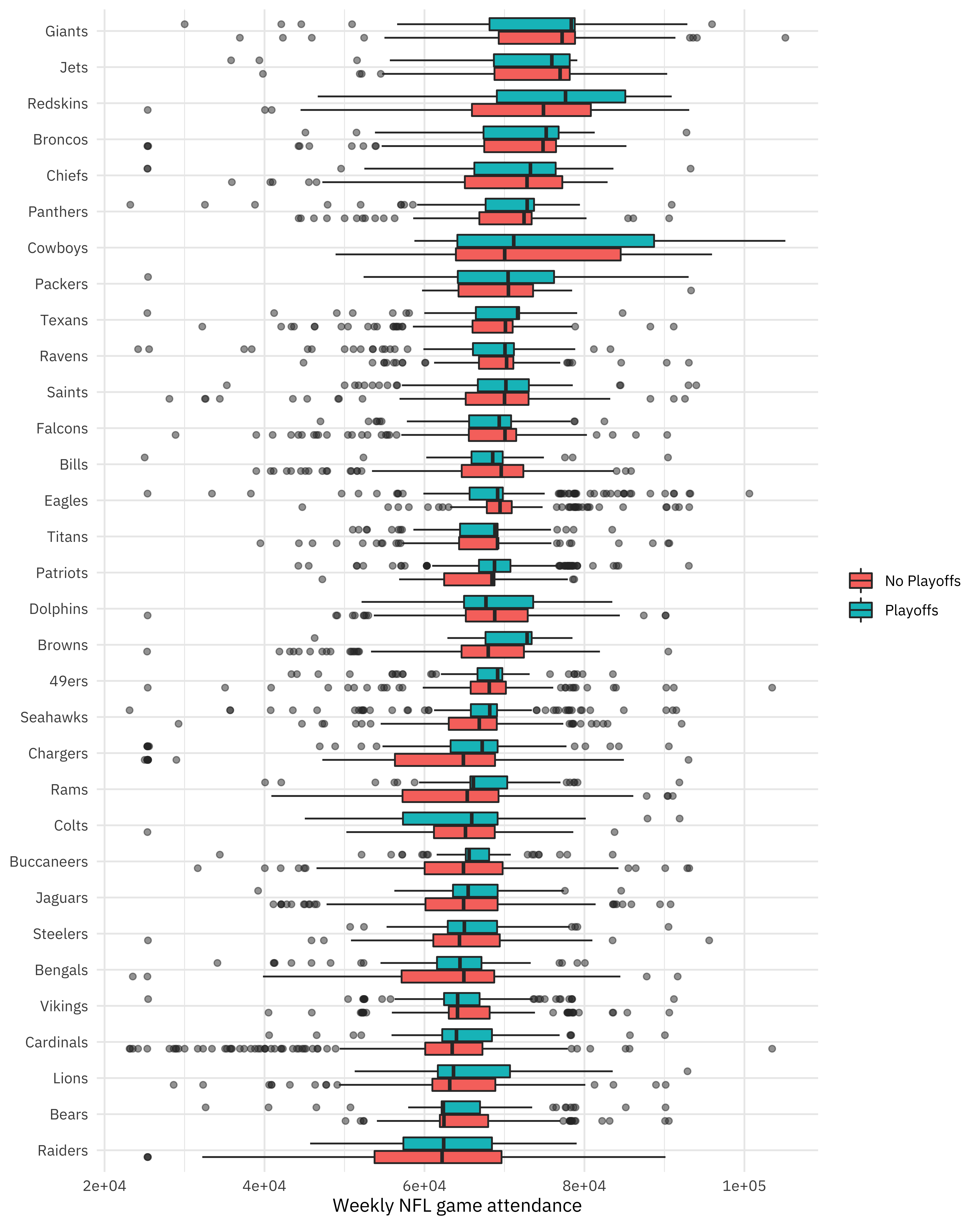
Notice that for the 32 teams in the NFL, we have years they all did and did not make the playoffs, which will be nice for modeling.

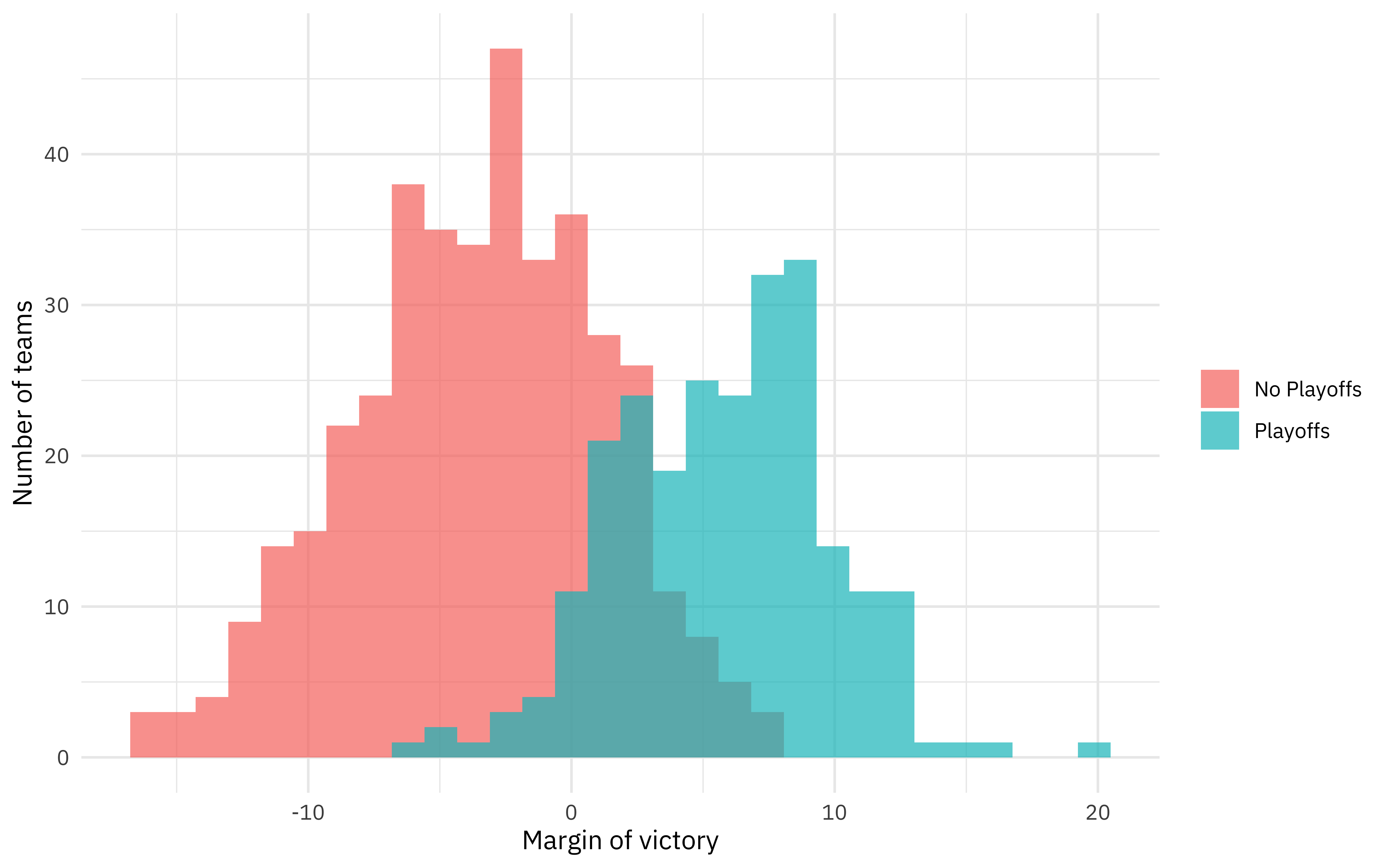
How much does margin_of_victory, a measure of points scored relative to points allowed, measure the same thing as getting to the playoffs?

attendance_joined %>%
  distinct(team_name, year, margin_of_victory, playoffs) %>%
  ggplot(aes(margin_of_victory, fill = playoffs)) +
  geom_histogram(position = "identity", alpha = 0.7) +
  labs(
    x = "Margin of victory",
    y = "Number of teams",
    fill = NULL
  )

Are there changes with the week of the season?

attendance_joined %>%
  mutate(week = factor(week)) %>%
  ggplot(aes(week, weekly_attendance, fill = week)) +
  geom_boxplot(show.legend = FALSE, outlier.alpha = 0.5) +
  labs(
    x = "Week of NFL season",
    y = "Weekly NFL game attendance"
  )

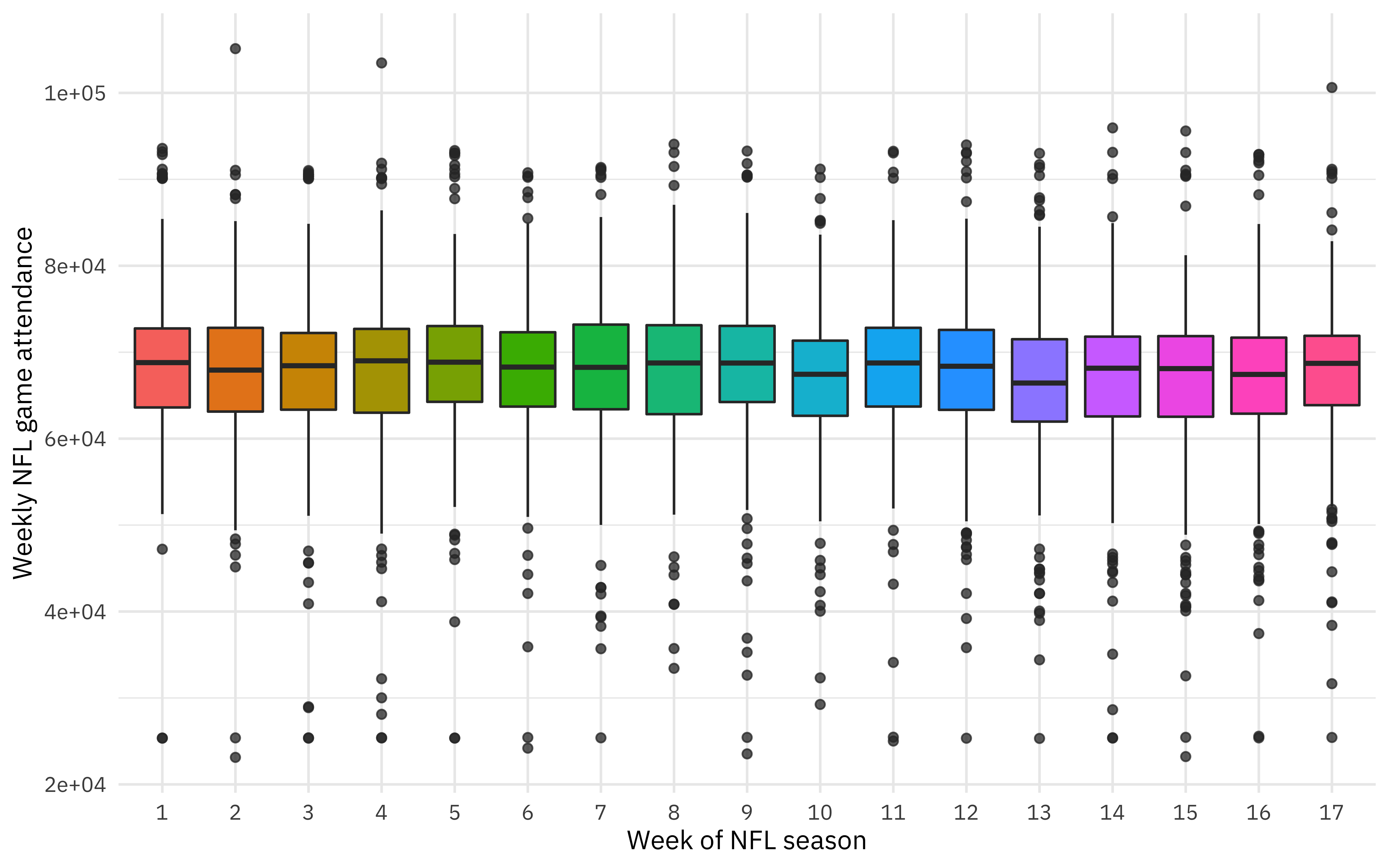
Maybe a bit.

This is some initial exploratory data analysis for this dataset, always an important part of a modeling task. To see more examples of EDA for this dataset, you can see the amazing work that folks share on Twitter. The next step for us here is to create a dataset for modeling.

• Let’s remove the weeks that each team did not play (where the weekly attendance is NA).
• Let’s only keep columns for modeling that we want to use for modeling. For example, we will keep margin_of_victory and strength_of_schedule, but not simple_rating which is the sum of those first two quantities.

attendance_df <- attendance_joined %>%
  filter(!is.na(weekly_attendance)) %>%
  select(
    weekly_attendance, team_name, year, week,
    margin_of_victory, strength_of_schedule, playoffs
  )

attendance_df

## # A tibble: 10,208 x 7
##    weekly_attendan… team_name  year  week margin_of_victo… strength_of_sch…
##               <dbl> <chr>     <dbl> <dbl>            <dbl>            <dbl>
##  1            77434 Cardinals  2000     1            -14.6             -0.7
##  2            66009 Cardinals  2000     2            -14.6             -0.7
##  3            71801 Cardinals  2000     4            -14.6             -0.7
##  4            66985 Cardinals  2000     5            -14.6             -0.7
##  5            44296 Cardinals  2000     6            -14.6             -0.7
##  6            38293 Cardinals  2000     7            -14.6             -0.7
##  7            62981 Cardinals  2000     8            -14.6             -0.7
##  8            35286 Cardinals  2000     9            -14.6             -0.7
##  9            52244 Cardinals  2000    10            -14.6             -0.7
## 10            64223 Cardinals  2000    11            -14.6             -0.7
## # … with 10,198 more rows, and 1 more variable: playoffs <chr>

Build simple models

Now it is time to load the tidymodels metapackage! 💪 The first step here is to split our data into training and testing tests. We can use initial_split() to create these datasets, divided so that they each have about the same number of examples of teams that went on to the playoffs.

library(tidymodels)

set.seed(1234)
attendance_split <- attendance_df %>%
  initial_split(strata = playoffs)

nfl_train <- training(attendance_split)
nfl_test <- testing(attendance_split)

Now we can specify and then fit our models. One of the significant problems that tidymodels solves is how so many modeling packages and functions in R have different inputs, calling sequences, and outputs. The code below might look like overkill to fit linear regression using OLS, but we can use the same framework to fit a regression model using Stan, using regularization, etc. The functions in tidymodels are designed to be composable and consistent.

lm_spec <- linear_reg() %>%
  set_engine(engine = "lm")

lm_spec

## Linear Regression Model Specification (regression)
##
## Computational engine: lm

lm_fit <- lm_spec %>%
  fit(weekly_attendance ~ .,
    data = nfl_train
  )

lm_fit

## parsnip model object
##
## Fit time:  16ms
##
## Call:
## stats::lm(formula = formula, data = data)
##
## Coefficients:
##          (Intercept)        team_nameBears      team_nameBengals
##            -81107.86              -2879.80              -4875.47
##       team_nameBills      team_nameBroncos       team_nameBrowns
##              -361.08               2805.24               -324.11
##  team_nameBuccaneers    team_nameCardinals     team_nameChargers
##             -3063.65              -6139.80              -6489.31
##      team_nameChiefs        team_nameColts      team_nameCowboys
##              1974.33              -3392.79               6068.70
##    team_nameDolphins       team_nameEagles      team_nameFalcons
##               139.68               1259.16               -204.17
##      team_nameGiants      team_nameJaguars         team_nameJets
##              5447.10              -3095.46               4044.23
##       team_nameLions      team_namePackers     team_namePanthers
##             -3480.69               1114.11               1227.32
##    team_namePatriots      team_nameRaiders         team_nameRams
##              -214.20              -6324.74              -2884.85
##      team_nameRavens     team_nameRedskins       team_nameSaints
##              -398.90               6447.07                380.98
##    team_nameSeahawks     team_nameSteelers       team_nameTexans
##             -1405.89              -3567.81                264.07
##      team_nameTitans      team_nameVikings                  year
##             -1118.23              -3183.08                 74.73
##                 week     margin_of_victory  strength_of_schedule
##               -72.83                137.58                230.74
##     playoffsPlayoffs
##              -427.94

So that’s one model! Let’s fit another one.

rf_spec <- rand_forest(mode = "regression") %>%
  set_engine("ranger")

rf_spec

## Random Forest Model Specification (regression)
##
## Computational engine: ranger

rf_fit <- rf_spec %>%
  fit(weekly_attendance ~ .,
    data = nfl_train
  )

rf_fit

## parsnip model object
##
## Fit time:  2.2s
## Ranger result
##
## Call:
##  ranger::ranger(formula = formula, data = data, num.threads = 1,      verbose = FALSE, seed = sample.int(10^5, 1))
##
## Type:                             Regression
## Number of trees:                  500
## Sample size:                      7656
## Number of independent variables:  6
## Mtry:                             2
## Target node size:                 5
## Variable importance mode:         none
## Splitrule:                        variance
## OOB prediction error (MSE):       74737868
## R squared (OOB):                  0.08217606

Notice that we have fit both of these models using nfl_train, the training data. We haven’t touched the testing data during training.

Evaluate models

When it’s time to evaluate our models (to estimate how well our models will perform on new data), then we will look at nfl_test. We can predict() what the weekly attendance will be for both the training data and the testing data using both the OLS and random forest models. One of the goals of tidymodels is to be able to use code like the following in predictable, consistent ways for many kinds of models, and to use existing well-suited tidyverse tools for these kinds of tasks.

results_train <- lm_fit %>%
  predict(new_data = nfl_train) %>%
  mutate(
    truth = nfl_train$weekly_attendance,
    model = "lm"
  ) %>%
  bind_rows(rf_fit %>%
    predict(new_data = nfl_train) %>%
    mutate(
      truth = nfl_train$weekly_attendance,
      model = "rf"
    ))

results_test <- lm_fit %>%
  predict(new_data = nfl_test) %>%
  mutate(
    truth = nfl_test$weekly_attendance,
    model = "lm"
  ) %>%
  bind_rows(rf_fit %>%
    predict(new_data = nfl_test) %>%
    mutate(
      truth = nfl_test$weekly_attendance,
      model = "rf"
    ))

For this regression model, let’s look at the rmse for what we’ve done so far.

results_train %>%
  group_by(model) %>%
  rmse(truth = truth, estimate = .pred)

## # A tibble: 2 x 4
##   model .metric .estimator .estimate
##   <chr> <chr>   <chr>          <dbl>
## 1 lm    rmse    standard       8307.
## 2 rf    rmse    standard       6102.

results_test %>%
  group_by(model) %>%
  rmse(truth = truth, estimate = .pred)

## # A tibble: 2 x 4
##   model .metric .estimator .estimate
##   <chr> <chr>   <chr>          <dbl>
## 1 lm    rmse    standard       8351.
## 2 rf    rmse    standard       8582.

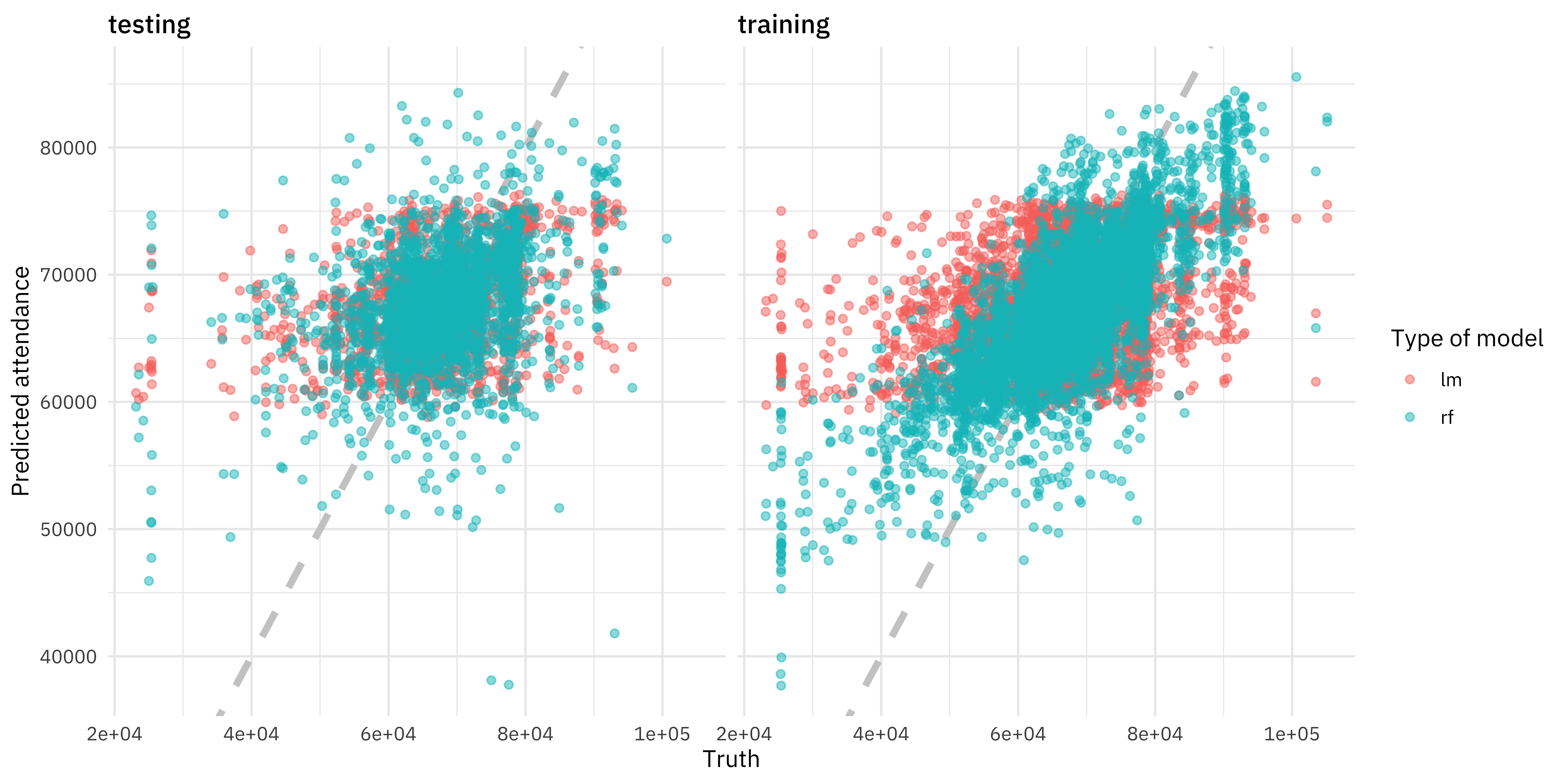
If we look at the training data, the random forest model performed much better than the linear model; the rmse is much lower. However, the same cannot be said for the testing data! 😭 The metric for training and testing for the linear model is about the same, meaning that we have not overfit. For the random forest model, the rmse is higher for the testing data than for the training data, by quite a lot. Our training data is not giving us a good idea of how our model is going to perform, and this powerful ML algorithm has overfit to this dataset.

Let’s visualize our sad situation.

results_test %>%
  mutate(train = "testing") %>%
  bind_rows(results_train %>%
    mutate(train = "training")) %>%
  ggplot(aes(truth, .pred, color = model)) +
  geom_abline(lty = 2, color = "gray80", size = 1.5) +
  geom_point(alpha = 0.5) +
  facet_wrap(~train) +
  labs(
    x = "Truth",
    y = "Predicted attendance",
    color = "Type of model"
  )

Let’s try this again!

We made not such a great decision in the previous section; we expected the random forest model evaluated one time on the whole training set to help us understand something about how it would perform on new data. This would be a reasonable expectation for the linear model, but not for the random forest. Fortunately, we have some options. We can resample the training set to produce an estimate of how the model will perform. Let’s divide our training set nfl_train into folds (say, 10) and fit 10 versions of our model (each one trained on nine folds and evaluated on one heldout fold). Then let’s measure how well our model(s) performs. The function vfold_cv() creates folds for cross-validation, the function fit_resamples() fits models to resamples such as these (to measure performance), and then we can collect_metrics() from the result.

set.seed(1234)
nfl_folds <- vfold_cv(nfl_train, strata = playoffs)

rf_res <- fit_resamples(
  weekly_attendance ~ .,
  rf_spec,
  nfl_folds,
  control = control_resamples(save_pred = TRUE)
)

rf_res %>%
  collect_metrics()

## # A tibble: 2 x 5
##   .metric .estimator     mean     n   std_err
##   <chr>   <chr>         <dbl> <int>     <dbl>
## 1 rmse    standard   8255.       10 115.
## 2 rsq     standard      0.164    10   0.00988

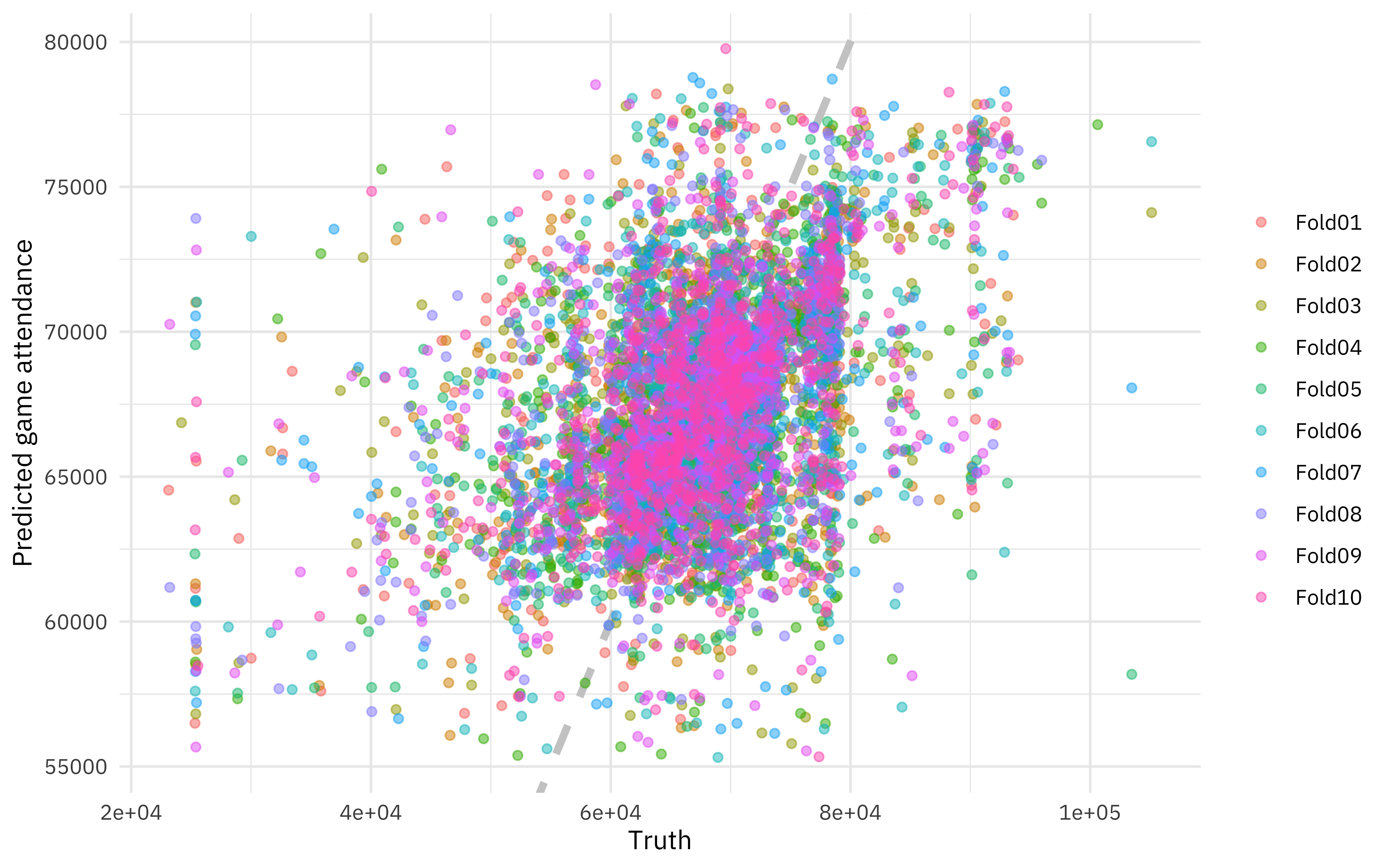
Remember that this is still the training dataset. We would take this step instead of the chunk above with predict(new_data = nfl_train), and we would still compare to how the model performs on the testing data. Notice that now we have a realistic estimate from the training data that is close to the testing data! We can even visualize our model results for the resamples.

rf_res %>%
  unnest(.predictions) %>%
  ggplot(aes(weekly_attendance, .pred, color = id)) +
  geom_abline(lty = 2, color = "gray80", size = 1.5) +
  geom_point(alpha = 0.5) +
  labs(
    x = "Truth",
    y = "Predicted game attendance",
    color = NULL
  )

Summary

Let me know if you have questions or feedback about this introduction to tidymodels and how to get started. I hope to do some more screencasts and blog posts about getting started with tidymodels, perhaps with more #TidyTuesday data!