LASSO regression using tidymodels and #TidyTuesday data for The Office

I’ve been publishing screencasts demonstrating how to use the tidymodels framework, from first steps in modeling to how to tune more complex models. Today, I’m using this week’s #TidyTuesday dataset on The Office to show how to build a lasso regression model and choose regularization parameters!

Here is the code I used in the video, for those who prefer reading instead of or in addition to video.

Explore the data

Our modeling goal here is to predict the IMDB ratings for episodes of The Office based on the other characteristics of the episodes in the #TidyTuesday dataset. There are two datasets, one with the ratings and one with information like director, writer, and which character spoke which line. The episode numbers and titles are not consistent between them, so we can use regular expressions to do a better job of matching the datasets up for joining.

library(tidyverse)

ratings_raw <- readr::read_csv("https://raw.githubusercontent.com/rfordatascience/tidytuesday/master/data/2020/2020-03-17/office_ratings.csv")

remove_regex <- "[:punct:]|[:digit:]|parts |part |the |and"

office_ratings <- ratings_raw %>%
  transmute(
    episode_name = str_to_lower(title),
    episode_name = str_remove_all(episode_name, remove_regex),
    episode_name = str_trim(episode_name),
    imdb_rating
  )

office_info <- schrute::theoffice %>%
  mutate(
    season = as.numeric(season),
    episode = as.numeric(episode),
    episode_name = str_to_lower(episode_name),
    episode_name = str_remove_all(episode_name, remove_regex),
    episode_name = str_trim(episode_name)
  ) %>%
  select(season, episode, episode_name, director, writer, character)

office_info

## # A tibble: 55,130 x 6
##    season episode episode_name director   writer                       character
##     <dbl>   <dbl> <chr>        <chr>      <chr>                        <chr>
##  1      1       1 pilot        Ken Kwapis Ricky Gervais;Stephen Merch… Michael
##  2      1       1 pilot        Ken Kwapis Ricky Gervais;Stephen Merch… Jim
##  3      1       1 pilot        Ken Kwapis Ricky Gervais;Stephen Merch… Michael
##  4      1       1 pilot        Ken Kwapis Ricky Gervais;Stephen Merch… Jim
##  5      1       1 pilot        Ken Kwapis Ricky Gervais;Stephen Merch… Michael
##  6      1       1 pilot        Ken Kwapis Ricky Gervais;Stephen Merch… Michael
##  7      1       1 pilot        Ken Kwapis Ricky Gervais;Stephen Merch… Michael
##  8      1       1 pilot        Ken Kwapis Ricky Gervais;Stephen Merch… Pam
##  9      1       1 pilot        Ken Kwapis Ricky Gervais;Stephen Merch… Michael
## 10      1       1 pilot        Ken Kwapis Ricky Gervais;Stephen Merch… Pam
## # … with 55,120 more rows

We are going to use several different kinds of features for modeling. First, let’s find out how many times characters speak per episode.

characters <- office_info %>%
  count(episode_name, character) %>%
  add_count(character, wt = n, name = "character_count") %>%
  filter(character_count > 800) %>%
  select(-character_count) %>%
  pivot_wider(
    names_from = character,
    values_from = n,
    values_fill = list(n = 0)
  )

characters

## # A tibble: 185 x 16
##    episode_name  Andy Angela Darryl Dwight   Jim Kelly Kevin Michael Oscar   Pam
##    <chr>        <int>  <int>  <int>  <int> <int> <int> <int>   <int> <int> <int>
##  1 a benihana …    28     37      3     61    44     5    14     108     1    57
##  2 aarm            44     39     30     87    89     0    30       0    28    34
##  3 after hours     20     11     14     60    55     8     4       0    10    15
##  4 alliance         0      7      0     47    49     0     3      68    14    22
##  5 angry y         53      7      5     16    19    13     9       0     7    29
##  6 baby shower     13     13      9     35    27     2     4      79     3    25
##  7 back from v…     3      4      6     22    25     0     5      70     0    33
##  8 banker           1      2      0     17     0     0     2      44     0     5
##  9 basketball       0      3     15     25    21     0     1     104     2    14
## 10 beach games     18      8      0     38    22     9     5     105     5    23
## # … with 175 more rows, and 5 more variables: Phyllis <int>, Ryan <int>,
## #   Toby <int>, Erin <int>, Jan <int>

Next, let’s find which directors and writers are involved in each episode. I’m choosing here to combine this into one category in modeling, for a simpler model, since these are often the same individuals.

creators <- office_info %>%
  distinct(episode_name, director, writer) %>%
  pivot_longer(director:writer, names_to = "role", values_to = "person") %>%
  separate_rows(person, sep = ";") %>%
  add_count(person) %>%
  filter(n > 10) %>%
  distinct(episode_name, person) %>%
  mutate(person_value = 1) %>%
  pivot_wider(
    names_from = person,
    values_from = person_value,
    values_fill = list(person_value = 0)
  )

creators

## # A tibble: 135 x 14
##    episode_name `Ken Kwapis` `Greg Daniels` `B.J. Novak` `Paul Lieberste…
##    <chr>               <dbl>          <dbl>        <dbl>            <dbl>
##  1 pilot                   1              1            0                0
##  2 diversity d…            1              0            1                0
##  3 health care             0              0            0                1
##  4 basketball              0              1            0                0
##  5 hot girl                0              0            0                0
##  6 dundies                 0              1            0                0
##  7 sexual hara…            1              0            1                0
##  8 office olym…            0              0            0                0
##  9 fire                    1              0            1                0
## 10 halloween               0              1            0                0
## # … with 125 more rows, and 9 more variables: `Mindy Kaling` <dbl>, `Paul
## #   Feig` <dbl>, `Gene Stupnitsky` <dbl>, `Lee Eisenberg` <dbl>, `Jennifer
## #   Celotta` <dbl>, `Randall Einhorn` <dbl>, `Brent Forrester` <dbl>, `Jeffrey
## #   Blitz` <dbl>, `Justin Spitzer` <dbl>

Next, let’s find the season and episode number for each episode, and then finally let’s put it all together into one dataset for modeling.

office <- office_info %>%
  distinct(season, episode, episode_name) %>%
  inner_join(characters) %>%
  inner_join(creators) %>%
  inner_join(office_ratings %>%
    select(episode_name, imdb_rating)) %>%
  janitor::clean_names()

office

## # A tibble: 136 x 32
##    season episode episode_name  andy angela darryl dwight   jim kelly kevin
##     <dbl>   <dbl> <chr>        <int>  <int>  <int>  <int> <int> <int> <int>
##  1      1       1 pilot            0      1      0     29    36     0     1
##  2      1       2 diversity d…     0      4      0     17    25     2     8
##  3      1       3 health care      0      5      0     62    42     0     6
##  4      1       5 basketball       0      3     15     25    21     0     1
##  5      1       6 hot girl         0      3      0     28    55     0     5
##  6      2       1 dundies          0      1      1     32    32     7     1
##  7      2       2 sexual hara…     0      2      9     11    16     0     6
##  8      2       3 office olym…     0      6      0     55    55     0     9
##  9      2       4 fire             0     17      0     65    51     4     5
## 10      2       5 halloween        0     13      0     33    30     3     2
## # … with 126 more rows, and 22 more variables: michael <int>, oscar <int>,
## #   pam <int>, phyllis <int>, ryan <int>, toby <int>, erin <int>, jan <int>,
## #   ken_kwapis <dbl>, greg_daniels <dbl>, b_j_novak <dbl>,
## #   paul_lieberstein <dbl>, mindy_kaling <dbl>, paul_feig <dbl>,
## #   gene_stupnitsky <dbl>, lee_eisenberg <dbl>, jennifer_celotta <dbl>,
## #   randall_einhorn <dbl>, brent_forrester <dbl>, jeffrey_blitz <dbl>,
## #   justin_spitzer <dbl>, imdb_rating <dbl>

There are lots of great examples of EDA on Twitter; I especially encourage you to check out the screencast of my coauthor Dave, which is similar in spirit to the modeling I am showing here and includes more EDA. Just for kicks, let’s show one graph.

office %>%
  ggplot(aes(episode, imdb_rating, fill = as.factor(episode))) +
  geom_boxplot(show.legend = FALSE)

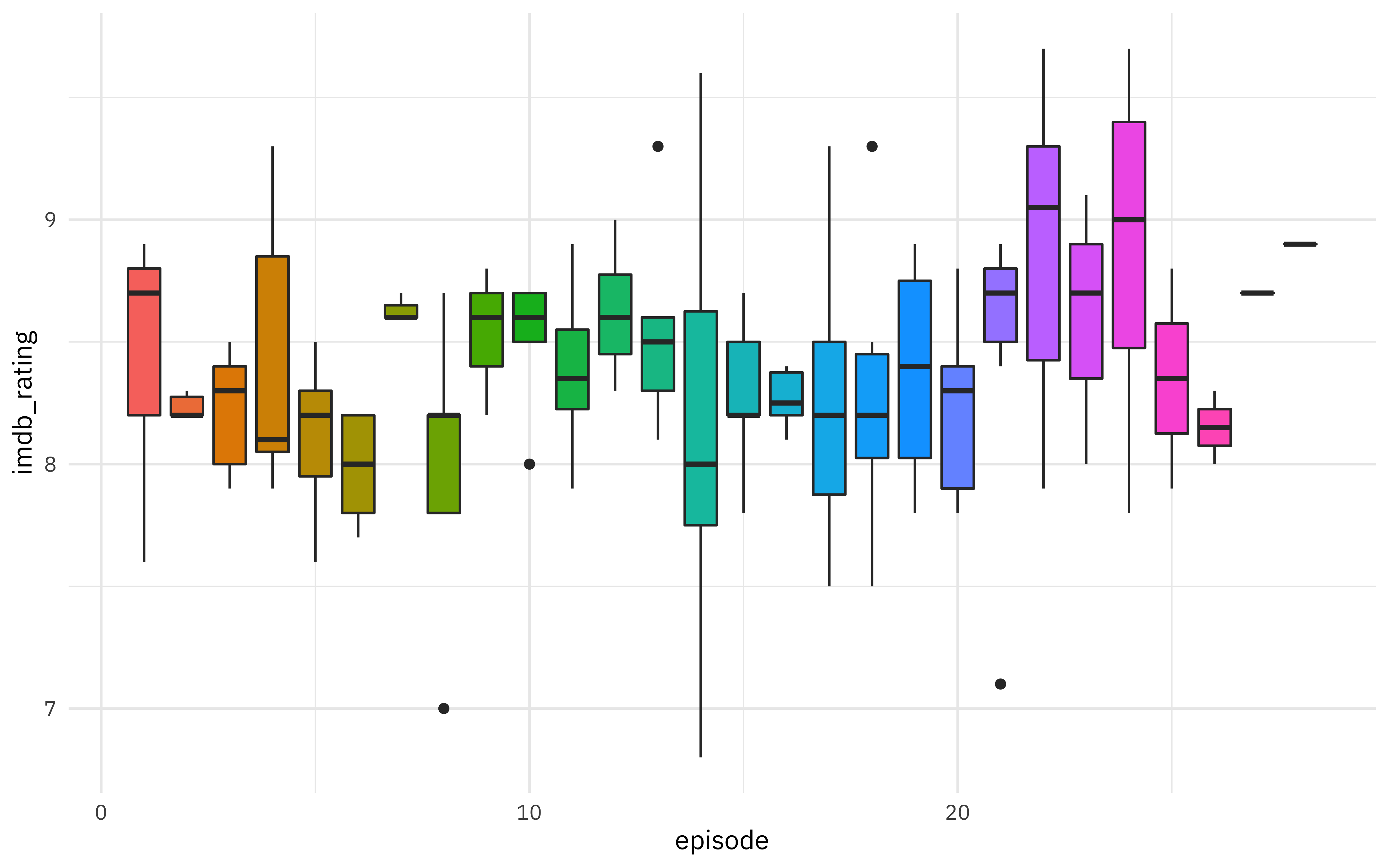
Ratings are higher for episodes later in the season. What else is associated with higher ratings? Let’s use lasso regression to find out! 🚀

Train a model

We can start by loading the tidymodels metapackage, and splitting our data into training and testing sets.

library(tidymodels)
office_split <- initial_split(office, strata = season)
office_train <- training(office_split)
office_test <- testing(office_split)

Then, we build a recipe for data preprocessing.

• First, we must tell the recipe() what our model is going to be (using a formula here) and what our training data is.
• Next, we update the role for episode_name, since this is a variable we might like to keep around for convenience as an identifier for rows but is not a predictor or outcome.
• Next, we remove any numeric variables that have zero variance.
• As a last step, we normalize (center and scale) the numeric variables. We need to do this because it’s important for lasso regularization.

The object office_rec is a recipe that has not been trained on data yet (for example, the centered and scaling has not been calculated) and office_prep is an object that has been trained on data. The reason I use strings_as_factors = FALSE here is that my ID column episode_name is of type character (as opposed to, say, integers).

office_rec <- recipe(imdb_rating ~ ., data = office_train) %>%
  update_role(episode_name, new_role = "ID") %>%
  step_zv(all_numeric(), -all_outcomes()) %>%
  step_normalize(all_numeric(), -all_outcomes())

office_prep <- office_rec %>%
  prep(strings_as_factors = FALSE)

Now it’s time to specify and then fit our models. Here I set up one model specification for lasso regression; I picked a value for penalty (sort of randomly) and I set mixture = 1 for lasso. I am using a workflow() in this example for convenience; these are objects that can help you manage modeling pipelines more easily, with pieces that fit together like Lego blocks. You can fit() a workflow, much like you can fit a model, and then you can pull out the fit object and tidy() it!

lasso_spec <- linear_reg(penalty = 0.1, mixture = 1) %>%
  set_engine("glmnet")

wf <- workflow() %>%
  add_recipe(office_rec)

lasso_fit <- wf %>%
  add_model(lasso_spec) %>%
  fit(data = office_train)

lasso_fit %>%
  pull_workflow_fit() %>%
  tidy()

## # A tibble: 1,576 x 5
##    term         step estimate lambda dev.ratio
##    <chr>       <dbl>    <dbl>  <dbl>     <dbl>
##  1 (Intercept)     1  8.36     0.195    0
##  2 (Intercept)     2  8.36     0.177    0.0244
##  3 jim             2  0.0174   0.177    0.0244
##  4 (Intercept)     3  8.36     0.162    0.0549
##  5 dwight          3  0.00254  0.162    0.0549
##  6 jim             3  0.0309   0.162    0.0549
##  7 michael         3  0.00800  0.162    0.0549
##  8 (Intercept)     4  8.36     0.147    0.0893
##  9 dwight          4  0.0116   0.147    0.0893
## 10 jim             4  0.0395   0.147    0.0893
## # … with 1,566 more rows

If you have used glmnet before, this is the familiar output where we can see (here, for the most regularized examples) what contributes to higher IMDB ratings.

Tune lasso parameters

So we fit one lasso model, but how do we know the right regularization parameter penalty? We can figure that out using resampling and tuning the model. Let’s build a set of bootstrap resamples, and set penalty = tune() instead of to a single value. We can use a function penalty() to set up an appropriate grid for this kind of regularization model.

set.seed(1234)
office_boot <- bootstraps(office_train, strata = season)

tune_spec <- linear_reg(penalty = tune(), mixture = 1) %>%
  set_engine("glmnet")

lambda_grid <- grid_regular(penalty(), levels = 50)

Now it’s time to tune the grid, using our workflow object.

doParallel::registerDoParallel()

set.seed(2020)
lasso_grid <- tune_grid(
  wf %>% add_model(tune_spec),
  resamples = office_boot,
  grid = lambda_grid
)

What results did we get?

lasso_grid %>%
  collect_metrics()

## # A tibble: 100 x 6
##     penalty .metric .estimator  mean     n std_err
##       <dbl> <chr>   <chr>      <dbl> <int>   <dbl>
##  1 1.00e-10 rmse    standard   0.588    25  0.0169
##  2 1.00e-10 rsq     standard   0.132    25  0.0212
##  3 1.60e-10 rmse    standard   0.588    25  0.0169
##  4 1.60e-10 rsq     standard   0.132    25  0.0212
##  5 2.56e-10 rmse    standard   0.588    25  0.0169
##  6 2.56e-10 rsq     standard   0.132    25  0.0212
##  7 4.09e-10 rmse    standard   0.588    25  0.0169
##  8 4.09e-10 rsq     standard   0.132    25  0.0212
##  9 6.55e-10 rmse    standard   0.588    25  0.0169
## 10 6.55e-10 rsq     standard   0.132    25  0.0212
## # … with 90 more rows

That’s nice, but I would rather see a visualization of performance with the regularization parameter.

lasso_grid %>%
  collect_metrics() %>%
  ggplot(aes(penalty, mean, color = .metric)) +
  geom_errorbar(aes(
    ymin = mean - std_err,
    ymax = mean + std_err
  ),
  alpha = 0.5
  ) +
  geom_line(size = 1.5) +
  facet_wrap(~.metric, scales = "free", nrow = 2) +
  scale_x_log10() +
  theme(legend.position = "none")

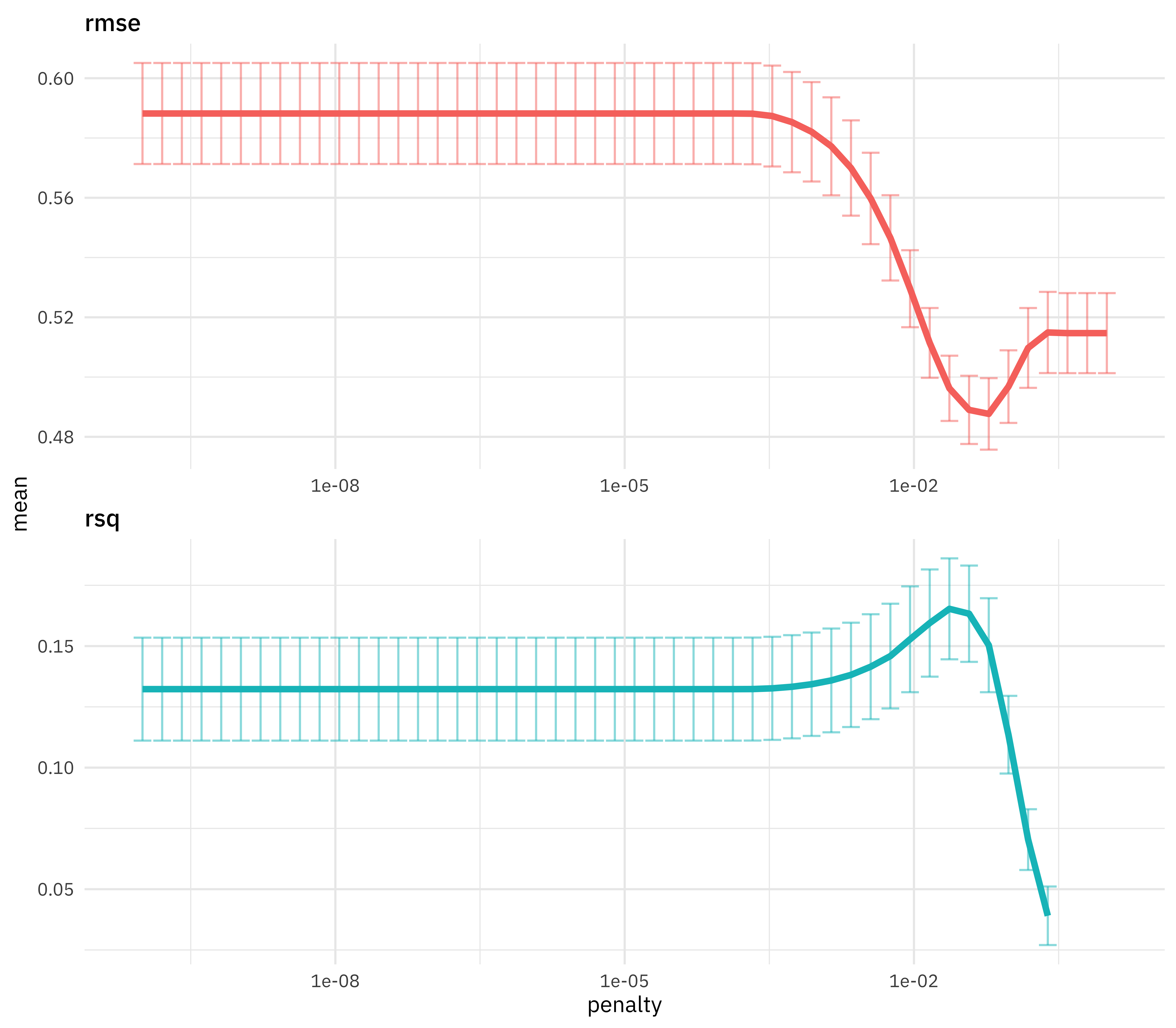
This is a great way to see that regularization helps this modeling a lot. We have a couple of options for choosing our final parameter, such as select_by_pct_loss() or select_by_one_std_err(), but for now let’s stick with just picking the lowest RMSE. After we have that parameter, we can finalize our workflow, i.e. update it with this value.

lowest_rmse <- lasso_grid %>%
  select_best("rmse", maximize = FALSE)

final_lasso <- finalize_workflow(
  wf %>% add_model(tune_spec),
  lowest_rmse
)

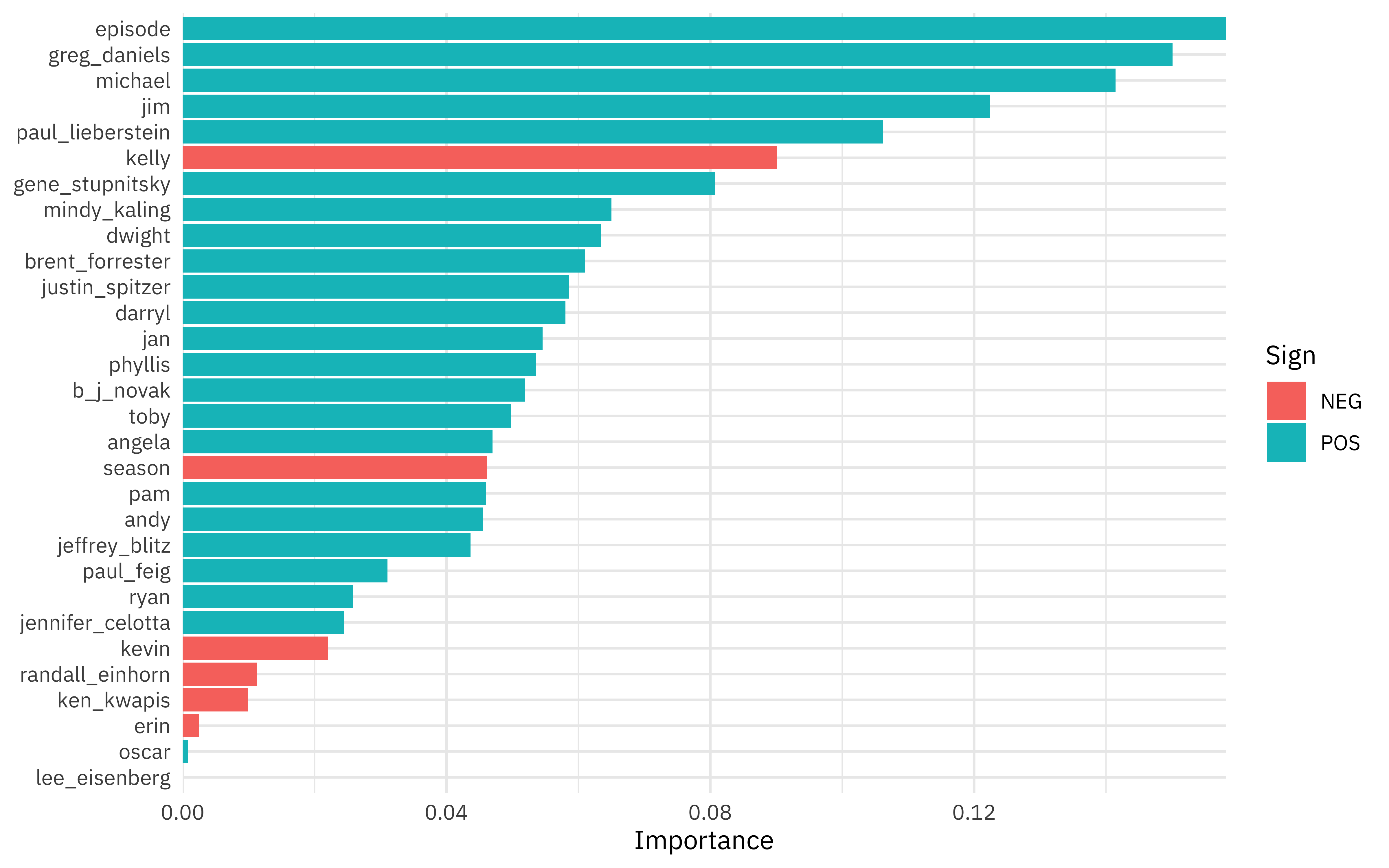
We can then fit this finalized workflow on our training data. While we’re at it, let’s see what the most important variables are using the vip package.

library(vip)

final_lasso %>%
  fit(office_train) %>%
  pull_workflow_fit() %>%
  vi(lambda = lowest_rmse$penalty) %>%
  mutate(
    Importance = abs(Importance),
    Variable = fct_reorder(Variable, Importance)
  ) %>%
  ggplot(aes(x = Importance, y = Variable, fill = Sign)) +
  geom_col() +
  scale_x_continuous(expand = c(0, 0)) +
  labs(y = NULL)

And then, finally, let’s return to our test data. The tune package has a function last_fit() which is nice for situations when you have tuned and finalized a model or workflow and want to fit it one last time on your training data and evaluate it on your testing data. You only have to pass this function your finalized model/workflow and your split.

last_fit(
  final_lasso,
  office_split
) %>%
  collect_metrics()

## # A tibble: 2 x 3
##   .metric .estimator .estimate
##   <chr>   <chr>          <dbl>
## 1 rmse    standard       0.436
## 2 rsq     standard       0.174