Tuning random forest hyperparameters with #TidyTuesday trees data
By Julia Silge in rstats tidymodels
March 26, 2020
I’ve been publishing
screencasts demonstrating how to use the tidymodels framework, from first steps in modeling to how to tune more complex models. Today, I’m using a
#TidyTuesday dataset from earlier this year on trees around San Francisco to show how to tune the hyperparameters of a random forest model and then use the final best model.
Here is the code I used in the video, for those who prefer reading instead of or in addition to video.
Explore the data
Our modeling goal here is to predict the legal status of the trees in San Francisco in the #TidyTuesday dataset. This isn’t this week’s dataset, but it’s one I have been wanting to return to. Because it seems almost wrong not to, we’ll be using a random forest model! 🌳
Let’s build a model to predict which trees are maintained by the
San Francisco Department of Public Works and which are not. We can use parse_number() to get a rough estimate of the size of the plot from the plot_size column. Instead of trying any imputation, we will just keep observations with no NA values.
library(tidyverse)

sf_trees <- read_csv("https://raw.githubusercontent.com/rfordatascience/tidytuesday/master/data/2020/2020-01-28/sf_trees.csv")

trees_df <- sf_trees %>%
  mutate(
    legal_status = case_when(
      legal_status == "DPW Maintained" ~ legal_status,
      TRUE ~ "Other"
    ),
    plot_size = parse_number(plot_size)
  ) %>%
  select(-address) %>%
  na.omit() %>%
  mutate_if(is.character, factor)
Let’s do a little exploratory data analysis before we fit models. How are these trees distributed across San Francisco?
trees_df %>%
  ggplot(aes(longitude, latitude, color = legal_status)) +
  geom_point(size = 0.5, alpha = 0.4) +
  labs(color = NULL)
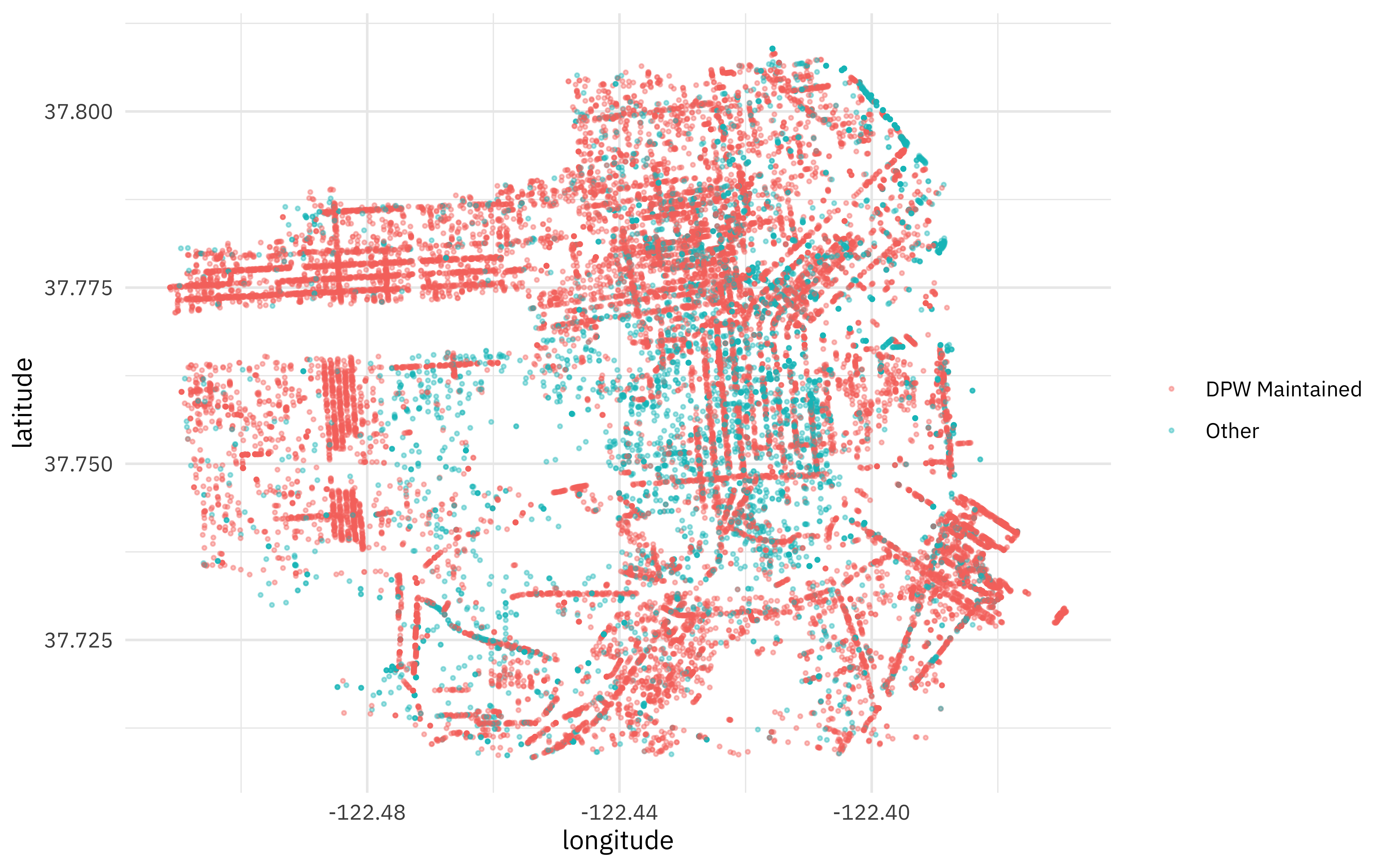
You can see streets! And there are definitely spatial differences by category.
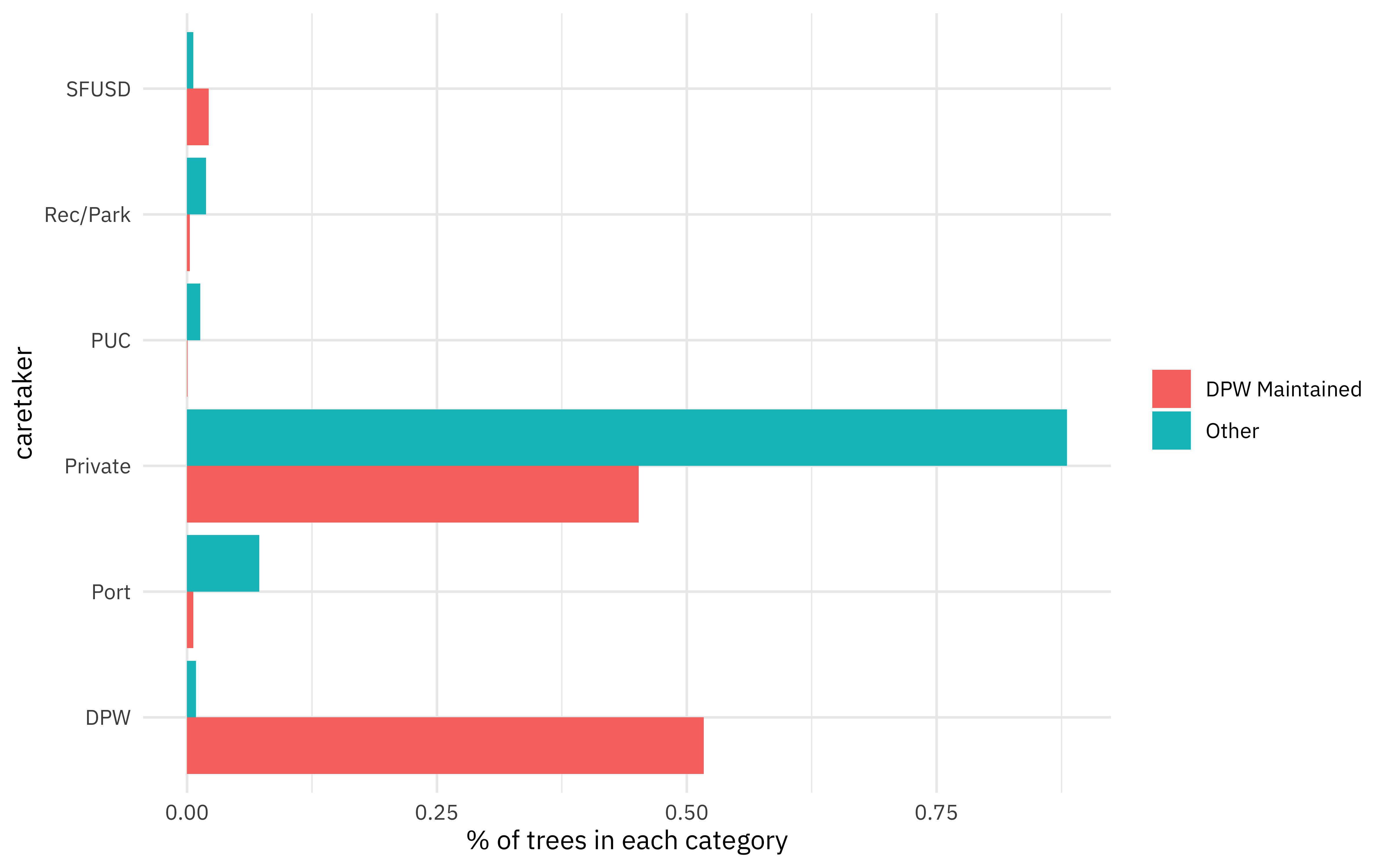
What relationships do we see with the caretaker of each tree?
trees_df %>%
  count(legal_status, caretaker) %>%
  add_count(caretaker, wt = n, name = "caretaker_count") %>%
  filter(caretaker_count > 50) %>%
  group_by(legal_status) %>%
  mutate(percent_legal = n / sum(n)) %>%
  ggplot(aes(percent_legal, caretaker, fill = legal_status)) +
  geom_col(position = "dodge") +
  labs(
    fill = NULL,
    x = "% of trees in each category"
  )
Build model
We can start by loading the tidymodels metapackage, and splitting our data into training and testing sets.
library(tidymodels)

set.seed(123)
trees_split <- initial_split(trees_df, strata = legal_status)
trees_train <- training(trees_split)
trees_test <- testing(trees_split)
Next we build a recipe for data preprocessing.
- First, we must tell the
recipe()what our model is going to be (using a formula here) and what our training data is. - Next, we update the role for
tree_id, since this is a variable we might like to keep around for convenience as an identifier for rows but is not a predictor or outcome. - Next, we use
step_other()to collapse categorical levels for species, caretaker, and the site info. Before this step, there were 300+ species! - The
datecolumn with when each tree was planted may be useful for fitting this model, but probably not the exact date, given how slowly trees grow. Let’s create a year feature from the date, and then remove the originaldatevariable. - There are many more DPW maintained trees than not, so let’s downsample the data for training.
The object tree_rec is a recipe that has not been trained on data yet (for example, which categorical levels should be collapsed has not been calculated) and tree_prep is an object that has been trained on data.
tree_rec <- recipe(legal_status ~ ., data = trees_train) %>%
  update_role(tree_id, new_role = "ID") %>%
  step_other(species, caretaker, threshold = 0.01) %>%
  step_other(site_info, threshold = 0.005) %>%
  step_dummy(all_nominal(), -all_outcomes()) %>%
  step_date(date, features = c("year")) %>%
  step_rm(date) %>%
  step_downsample(legal_status)

tree_prep <- prep(tree_rec)
juiced <- juice(tree_prep)
Now it’s time to create a model specification for a random forest where we will tune mtry (the number of predictors to sample at each split) and min_n (the number of observations needed to keep splitting nodes). These are hyperparameters that can’t be learned from data when training the model.
tune_spec <- rand_forest(
  mtry = tune(),
  trees = 1000,
  min_n = tune()
) %>%
  set_mode("classification") %>%
  set_engine("ranger")
Finally, let’s put these together in a
workflow(), which is a convenience container object for carrying around bits of models.
tune_wf <- workflow() %>%
  add_recipe(tree_rec) %>%
  add_model(tune_spec)
This workflow is ready to go. 🚀
Train hyperparameters
Now it’s time to tune the hyperparameters for a random forest model. First, let’s create a set of cross-validation resamples to use for tuning.
set.seed(234)
trees_folds <- vfold_cv(trees_train)
We can’t learn the right values when training a single model, but we can train a whole bunch of models and see which ones turn out best. We can use parallel processing to make this go faster, since the different parts of the grid are independent. Let’s use grid = 20 to choose 20 grid points automatically.
doParallel::registerDoParallel()

set.seed(345)
tune_res <- tune_grid(
  tune_wf,
  resamples = trees_folds,
  grid = 20
)

tune_res
## #  10-fold cross-validation
## # A tibble: 10 x 4
##    splits               id     .metrics          .notes
##    <list>               <chr>  <list>            <list>
##  1 <split [16.1K/1.8K]> Fold01 <tibble [40 × 5]> <tibble [0 × 1]>
##  2 <split [16.1K/1.8K]> Fold02 <tibble [40 × 5]> <tibble [0 × 1]>
##  3 <split [16.1K/1.8K]> Fold03 <tibble [40 × 5]> <tibble [0 × 1]>
##  4 <split [16.1K/1.8K]> Fold04 <tibble [40 × 5]> <tibble [0 × 1]>
##  5 <split [16.1K/1.8K]> Fold05 <tibble [40 × 5]> <tibble [0 × 1]>
##  6 <split [16.1K/1.8K]> Fold06 <tibble [40 × 5]> <tibble [0 × 1]>
##  7 <split [16.1K/1.8K]> Fold07 <tibble [40 × 5]> <tibble [0 × 1]>
##  8 <split [16.1K/1.8K]> Fold08 <tibble [40 × 5]> <tibble [0 × 1]>
##  9 <split [16.1K/1.8K]> Fold09 <tibble [40 × 5]> <tibble [0 × 1]>
## 10 <split [16.1K/1.8K]> Fold10 <tibble [40 × 5]> <tibble [0 × 1]>
How did this turn out? Let’s look at AUC.
tune_res %>%
  collect_metrics() %>%
  filter(.metric == "roc_auc") %>%
  select(mean, min_n, mtry) %>%
  pivot_longer(min_n:mtry,
    values_to = "value",
    names_to = "parameter"
  ) %>%
  ggplot(aes(value, mean, color = parameter)) +
  geom_point(show.legend = FALSE) +
  facet_wrap(~parameter, scales = "free_x") +
  labs(x = NULL, y = "AUC")
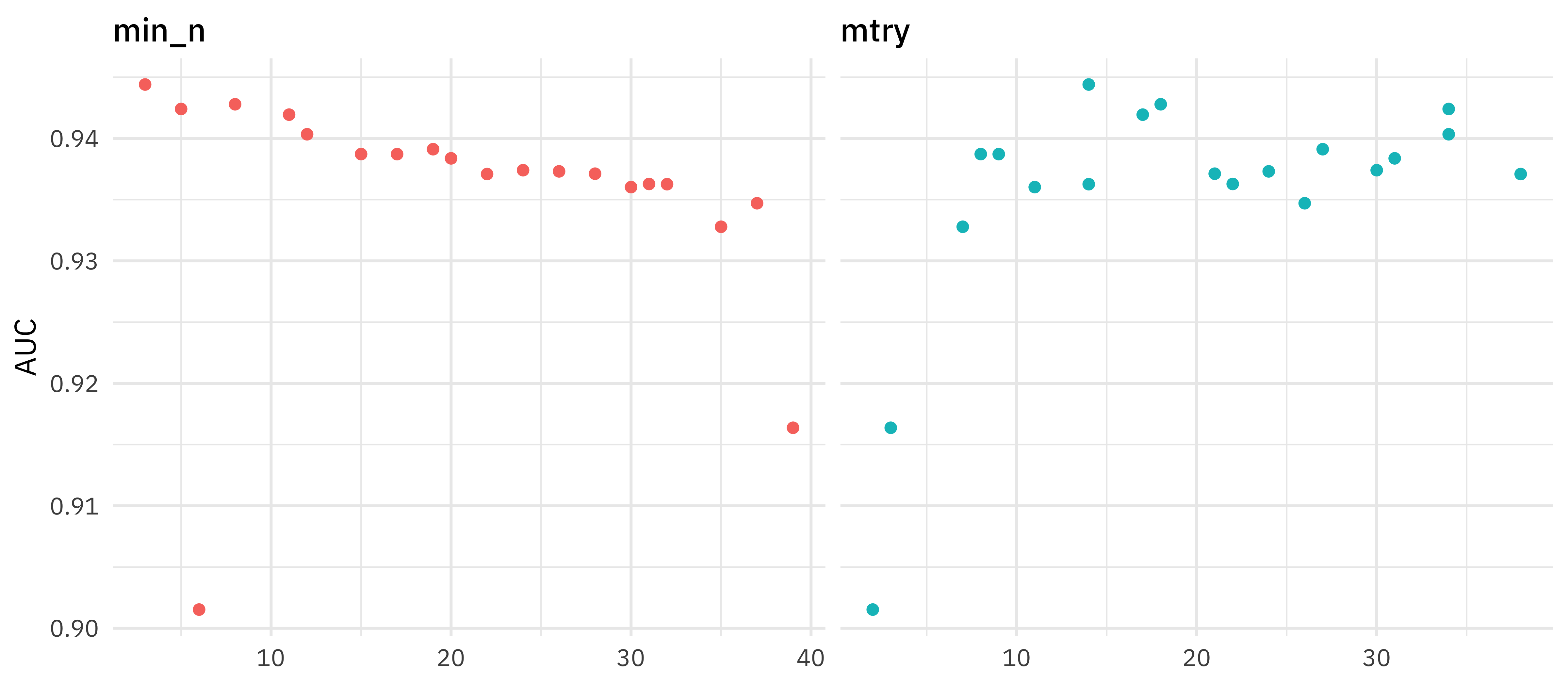
This grid did not involve every combination of min_n and mtry but we can get an idea of what is going on. It looks like higher values of mtry are good (above about 10) and lower values of min_n are good (below about 10). We can get a better handle on the hyperparameters by tuning one more time, this time using regular_grid(). Let’s set ranges of hyperparameters we want to try, based on the results from our initial tune.
rf_grid <- grid_regular(
  mtry(range = c(10, 30)),
  min_n(range = c(2, 8)),
  levels = 5
)

rf_grid
## # A tibble: 25 x 2
##     mtry min_n
##    <int> <int>
##  1    10     2
##  2    15     2
##  3    20     2
##  4    25     2
##  5    30     2
##  6    10     3
##  7    15     3
##  8    20     3
##  9    25     3
## 10    30     3
## # … with 15 more rows
We can tune one more time, but this time in a more targeted way with this rf_grid.
set.seed(456)
regular_res <- tune_grid(
  tune_wf,
  resamples = trees_folds,
  grid = rf_grid
)

regular_res
## #  10-fold cross-validation
## # A tibble: 10 x 4
##    splits               id     .metrics          .notes
##    <list>               <chr>  <list>            <list>
##  1 <split [16.1K/1.8K]> Fold01 <tibble [50 × 5]> <tibble [0 × 1]>
##  2 <split [16.1K/1.8K]> Fold02 <tibble [50 × 5]> <tibble [0 × 1]>
##  3 <split [16.1K/1.8K]> Fold03 <tibble [50 × 5]> <tibble [0 × 1]>
##  4 <split [16.1K/1.8K]> Fold04 <tibble [50 × 5]> <tibble [0 × 1]>
##  5 <split [16.1K/1.8K]> Fold05 <tibble [50 × 5]> <tibble [0 × 1]>
##  6 <split [16.1K/1.8K]> Fold06 <tibble [50 × 5]> <tibble [0 × 1]>
##  7 <split [16.1K/1.8K]> Fold07 <tibble [50 × 5]> <tibble [0 × 1]>
##  8 <split [16.1K/1.8K]> Fold08 <tibble [50 × 5]> <tibble [0 × 1]>
##  9 <split [16.1K/1.8K]> Fold09 <tibble [50 × 5]> <tibble [0 × 1]>
## 10 <split [16.1K/1.8K]> Fold10 <tibble [50 × 5]> <tibble [0 × 1]>
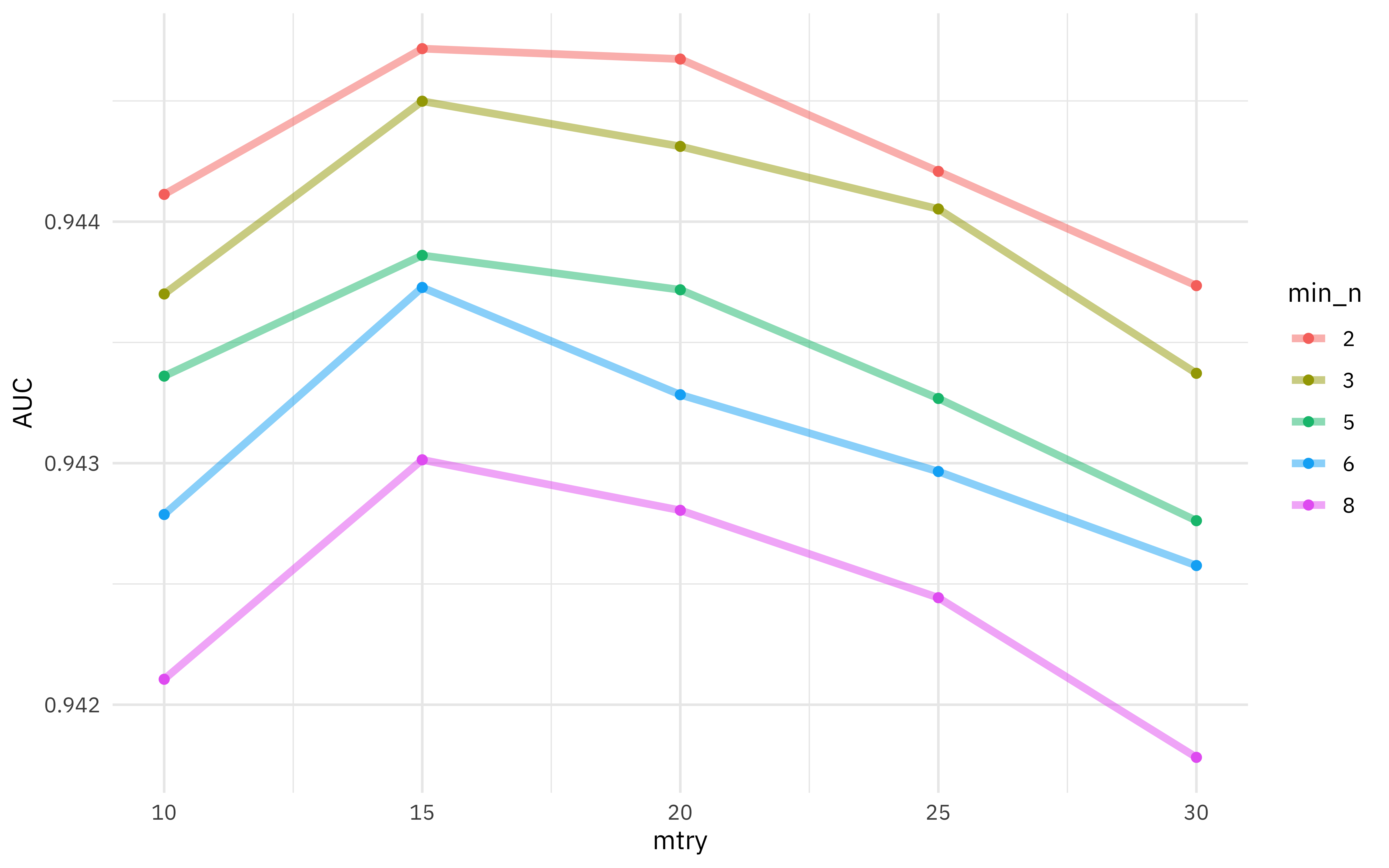
What the results look like now?
regular_res %>%
  collect_metrics() %>%
  filter(.metric == "roc_auc") %>%
  mutate(min_n = factor(min_n)) %>%
  ggplot(aes(mtry, mean, color = min_n)) +
  geom_line(alpha = 0.5, size = 1.5) +
  geom_point() +
  labs(y = "AUC")
Choosing the best model
It’s much more clear what the best model is now. We can identify it using the function select_best(), and then update our original model specification tune_spec to create our final model specification.
best_auc <- select_best(regular_res, "roc_auc")

final_rf <- finalize_model(
  tune_spec,
  best_auc
)

final_rf
## Random Forest Model Specification (classification)
##
## Main Arguments:
##   mtry = 15
##   trees = 1000
##   min_n = 2
##
## Computational engine: ranger
Let’s explore our final model a bit. What can we learn about variable importance, using the vip package?
library(vip)

final_rf %>%
  set_engine("ranger", importance = "permutation") %>%
  fit(legal_status ~ .,
    data = juice(tree_prep) %>% select(-tree_id)
  ) %>%
  vip(geom = "point")
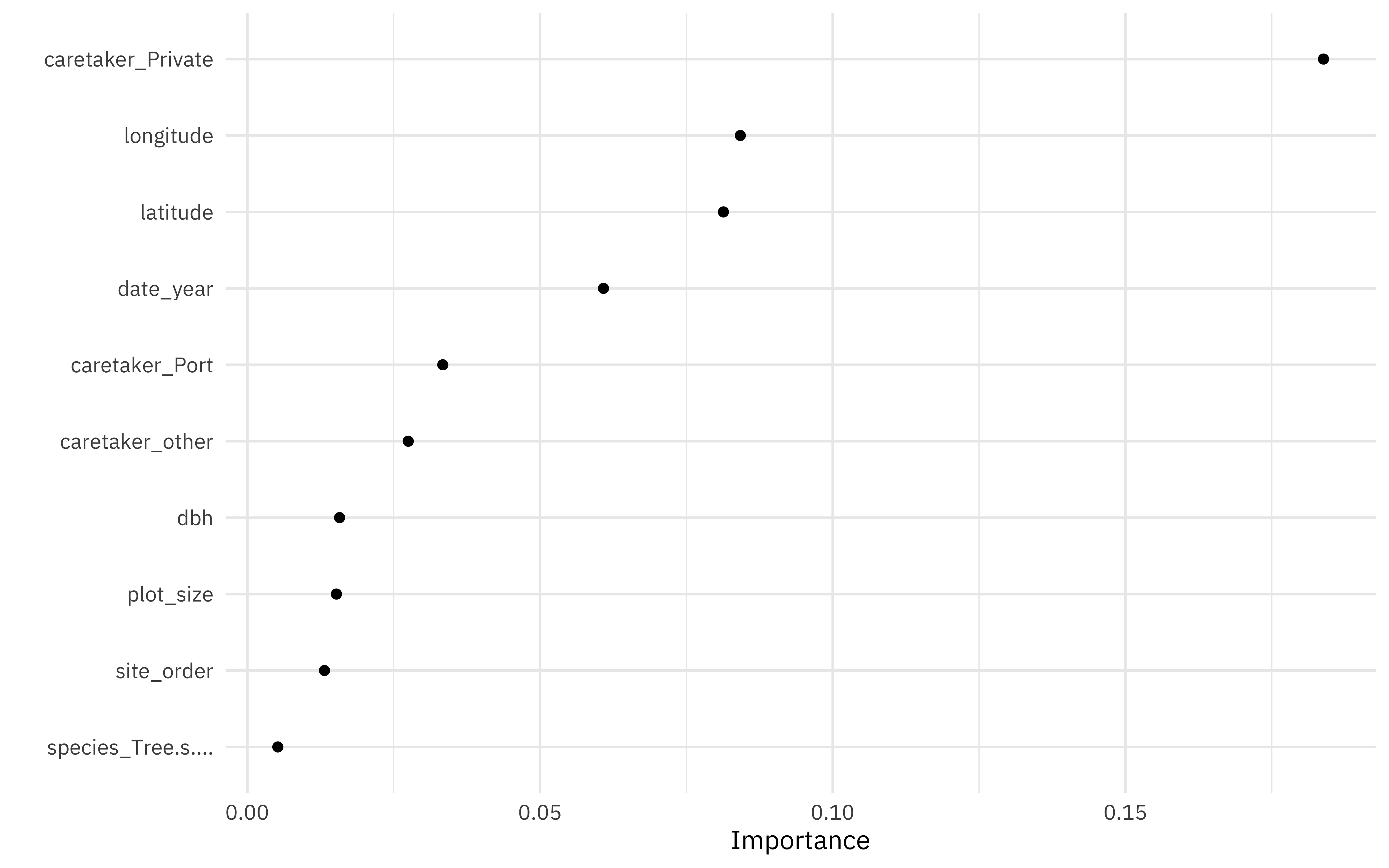
The private caretaker characteristic important in categorization, as is latitude and longitude. Interesting that year (i.e. age of the tree) is so important!
Let’s make a final workflow, and then fit one last time, using the convenience function
last_fit(). This function fits a final model on the entire training set and evaluates on the testing set. We just need to give this funtion our original train/test split.
final_wf <- workflow() %>%
  add_recipe(tree_rec) %>%
  add_model(final_rf)

final_res <- final_wf %>%
  last_fit(trees_split)

final_res %>%
  collect_metrics()
## # A tibble: 2 x 3
##   .metric  .estimator .estimate
##   <chr>    <chr>          <dbl>
## 1 accuracy binary         0.847
## 2 roc_auc  binary         0.949
The metrics for the test set look good and indicate we did not overfit during tuning.
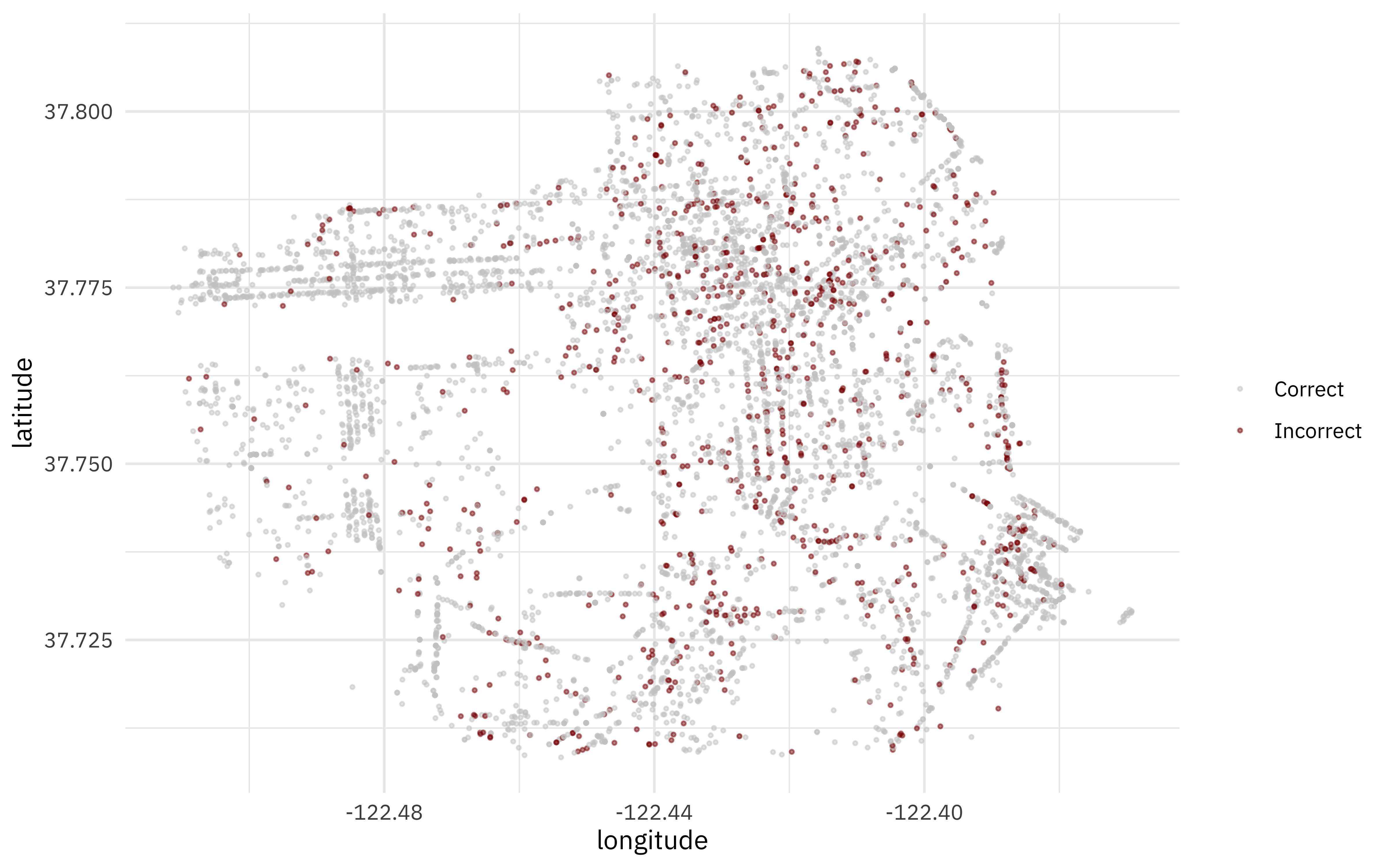
Let’s bind our testing results back to the original test set, and make one more map. Where in San Francisco are there more or less incorrectly predicted trees?
final_res %>%
  collect_predictions() %>%
  mutate(correct = case_when(
    legal_status == .pred_class ~ "Correct",
    TRUE ~ "Incorrect"
  )) %>%
  bind_cols(trees_test) %>%
  ggplot(aes(longitude, latitude, color = correct)) +
  geom_point(size = 0.5, alpha = 0.5) +
  labs(color = NULL) +
  scale_color_manual(values = c("gray80", "darkred"))
- Posted on:
- March 26, 2020
- Length:
- 8 minute read, 1662 words
- Categories:
- rstats tidymodels
- Tags:
- rstats tidymodels