Sliding windows for #TidyTuesday rents in San Francisco

This is the latest in my series of screencasts, but it is not about tidymodels this time around! I am stepping away from working on tidymodels to focus on MLOps tools full-time, so moving forward I’ll focus on a wider variety on topics in screencasts. An important part of managing deployed models is monitoring, and this involves computing model metrics at a given aggregation. I love to use the slider package by my coworker Davis Vaughan for this kind of task, and this screencast walks through how to use sliding window aggregation to analyze a recent #TidyTuesday dataset on rents in San Francisco. 🏙️

Here is the code I used in the video, for those who prefer reading instead of or in addition to video.

Load data

Our analysis goal is to understand how rents in San Francisco are changing over time. This dataset is from last month, but I didn’t get a chance to look at it then because of preparing for rstudio::conf()! Let’s filter down to apartments that are whole apartments (not a room for rent) and listings that are from the last 15 years or so.

library(tidyverse)

rent_raw <- read_csv('https://raw.githubusercontent.com/rfordatascience/tidytuesday/master/data/2022/2022-07-05/rent.csv')

rent <- rent_raw %>%
    filter(room_in_apt < 1, year > 2005) %>%
    select(date, price, beds, baths) %>%
    mutate(date = lubridate::ymd(date)) %>%
    arrange(date)

rent

## # A tibble: 144,261 × 4
##    date       price  beds baths
##    <date>     <dbl> <dbl> <dbl>
##  1 2006-01-01  1000     2     1
##  2 2006-01-01   900     1    NA
##  3 2006-01-01  1100     1     1
##  4 2006-01-01  1750     2    NA
##  5 2006-01-01  1050     2    NA
##  6 2006-01-01  2100     2    NA
##  7 2006-01-01   750     3    NA
##  8 2006-01-01  1195     0    NA
##  9 2006-01-01   600     1    NA
## 10 2006-01-01  1295     0     1
## # … with 144,251 more rows
## # ℹ Use `print(n = ...)` to see more rows

Compute a sliding mean

Let’s use the sliding_period_*() family of functions, since we have date information and want to aggregate in a date-aware way. These functions may reminder you of purrr::map() in that you can specify the type of the output and you pass in a function to use for the aggregation. How can we compute the mean price during each month?

library(slider)
slide_period_dbl(rent, rent$date, "month", ~ mean(.$price))

##   [1] 1702.348 1764.308 1680.277 1780.290 1741.493 1792.470 1937.523 1916.761
##   [9] 2158.055 1981.265 2000.490 1837.366 2863.852 1944.671 1886.720 1929.790
##  [17] 1949.142 2122.238 2145.564 2095.632 2213.338 2162.576 1836.880 1935.268
##  [25] 2093.470 2101.785 2158.061 2069.820 2321.663 1402.000 2053.995 2075.493
##  [33] 1923.436 1997.835 1810.720 2563.304 1668.604 1714.088 1877.848 2012.075
##  [41] 1414.392 1894.130 1850.200 2169.115 1988.202 1921.168 2494.451 2024.189
##  [49] 2171.402 2061.801 2052.503 2071.554 2142.095 2218.942 2173.790 2258.142
##  [57] 2367.558 2339.565 1932.022 1636.667 3000.000 2403.243 2392.396 2112.032
##  [65] 2304.910 2613.418 2471.167 2918.508 2783.562 2369.468 2964.150 3017.188
##  [73] 3008.525 2373.783 3307.472 2832.411 2687.975 2895.371 3381.402 2694.425
##  [81] 2733.273 2459.929 3014.436 2954.046 3004.527 3050.929 3268.769 2596.823
##  [89] 3051.025 3145.838 3156.274 2807.752 2883.929 2838.391 2867.761 2980.510
##  [97] 2807.714 3024.339 3128.416 2877.165 2896.006 3050.295 2949.307 3076.659
## [105] 3700.000 2904.348 3264.213 3044.426 2940.444 3041.136 2915.409 2876.117
## [113] 3071.498 2941.088 2982.688 2984.801 2993.061

Nice! But I think I would like this in a dataframe, with the date that belongs to each mean price and maybe also the number that was used for the aggregation. I think this is easiest if I write a little function:

mean_rent <- function(df) {
    summarize(df, date = min(date), rent = mean(price), n = n())
}

slide_period_dfr(rent, rent$date, "month", mean_rent)

## # A tibble: 117 × 3
##    date        rent     n
##    <date>     <dbl> <int>
##  1 2006-01-01 1702.  1323
##  2 2006-02-03 1764.  3125
##  3 2006-03-01 1680.  1315
##  4 2006-04-01 1780.  4996
##  5 2006-05-01 1741.  1391
##  6 2006-06-02 1792.  1816
##  7 2006-07-05 1938.  2711
##  8 2006-08-11 1917.  2189
##  9 2006-09-01 2158.   474
## 10 2006-10-18 1981.   185
## # … with 107 more rows
## # ℹ Use `print(n = ...)` to see more rows

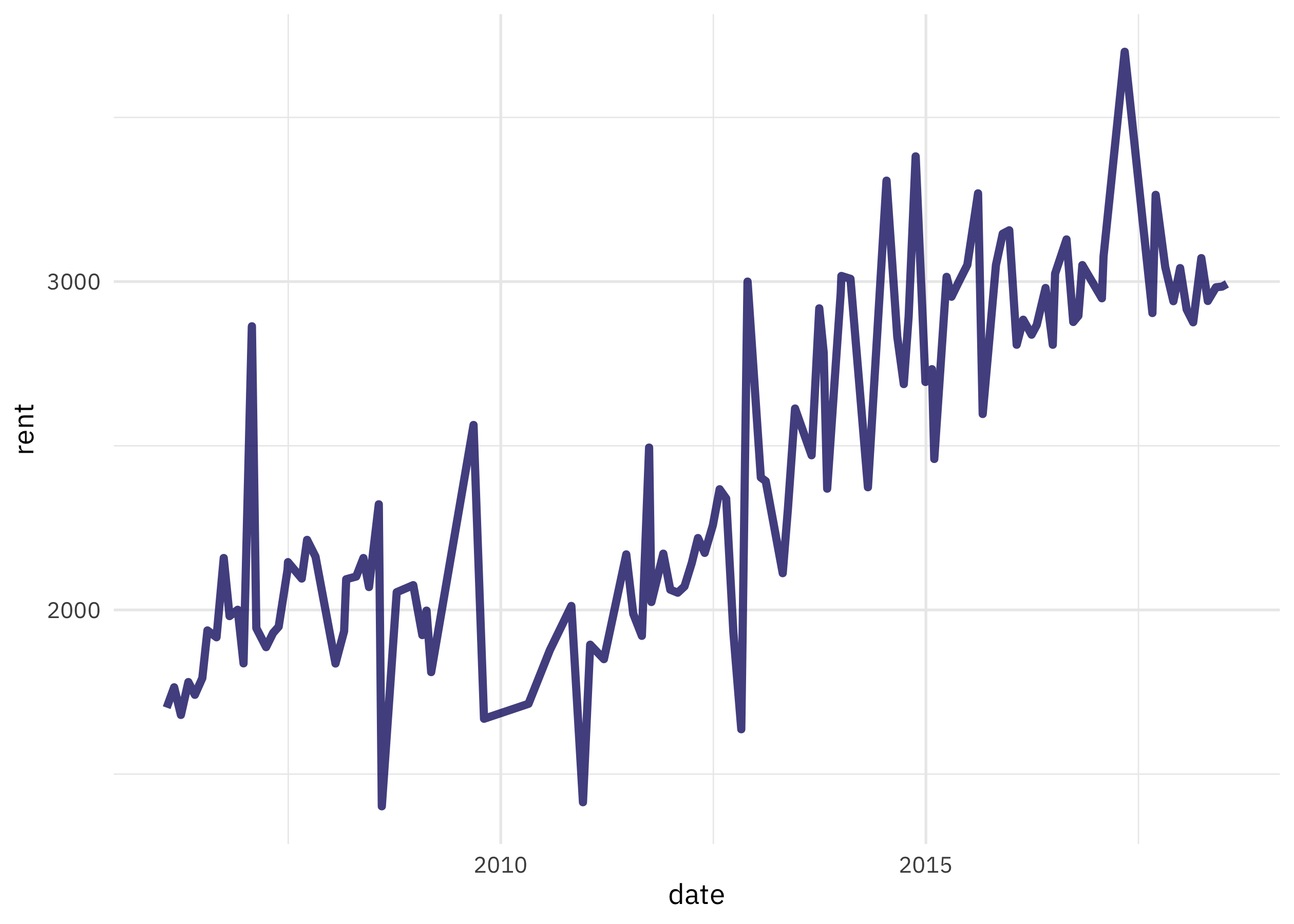
I could save this object, or I can just pipe it straight to ggplot2:

slide_period_dfr(rent, rent$date, "month", mean_rent) %>%
    ggplot(aes(date, rent)) +
    geom_line(size = 1.5, alpha = 0.8)

Now the real helpfulness of slider comes in when I want to more flexibly aggregate, with a more complex sliding window. Let’s use .before = 1, which makes a sliding window that includes both the current month and the previous month:

slide_period_dfr(rent, rent$date, "month", mean_rent, .before = 1) %>%
    ggplot(aes(date, rent)) +
    geom_line(size = 1.5, alpha = 0.8)

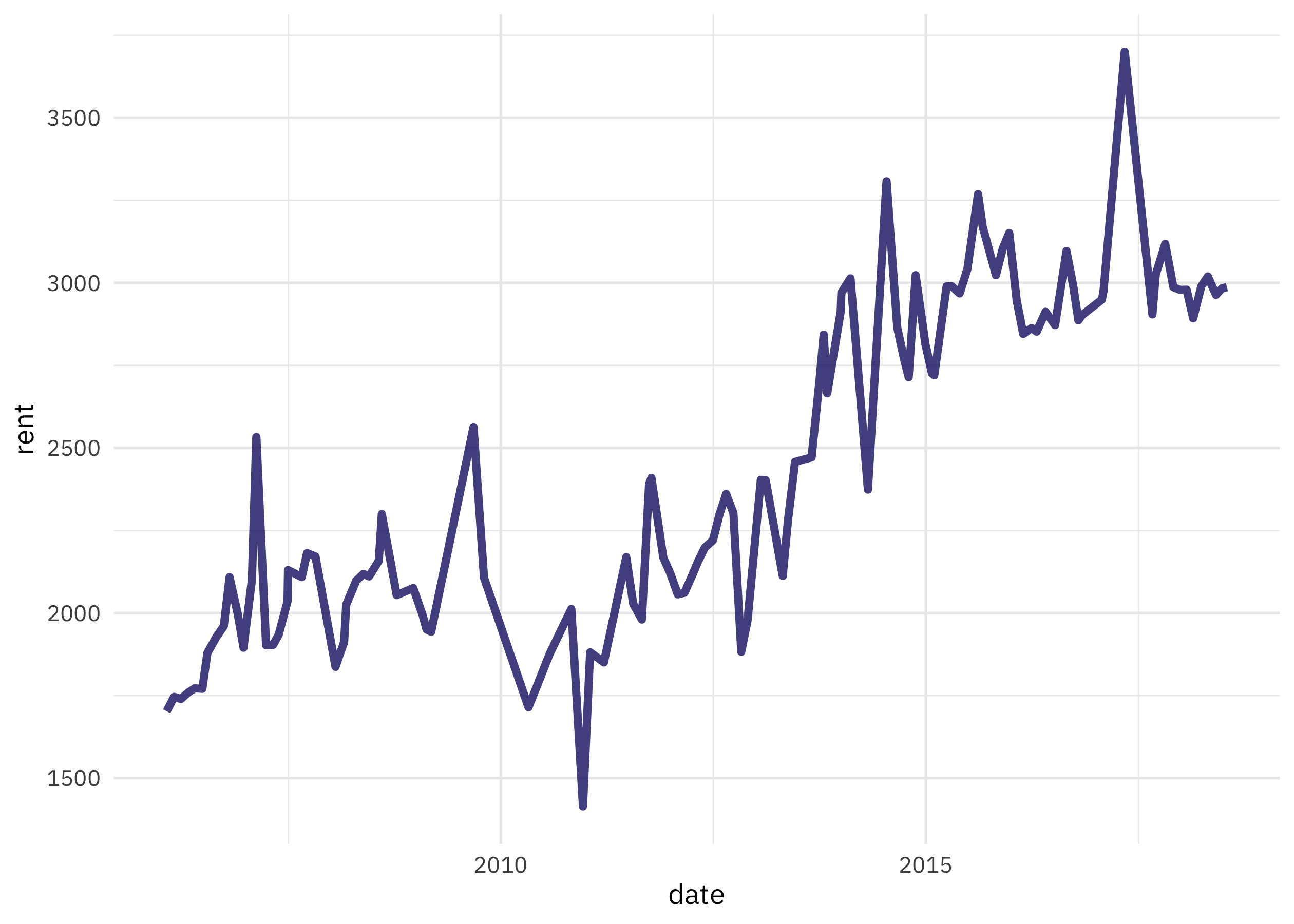
The main difference we see here is that the variation is smoothing out a bit, since we are taking the average over a longer time period.

Different sliding windows

What does it look like if we try different values for .before, from one previous month to six previous months?

tibble(.before = 1:6) %>%
    mutate(mean_rent = map(
        .before, 
        ~ slide_period_dfr(rent, rent$date, "month", mean_rent, .before = .x)
    )) %>%
    unnest(mean_rent) %>%
    ggplot(aes(date, rent, color = .before, group = .before)) +
    geom_line(alpha = 0.6, size = 1.5) +
    scale_color_viridis_c() +
    scale_y_continuous(labels = scales::dollar) +
    labs(x = NULL, color = "How many months\nin sliding window?")

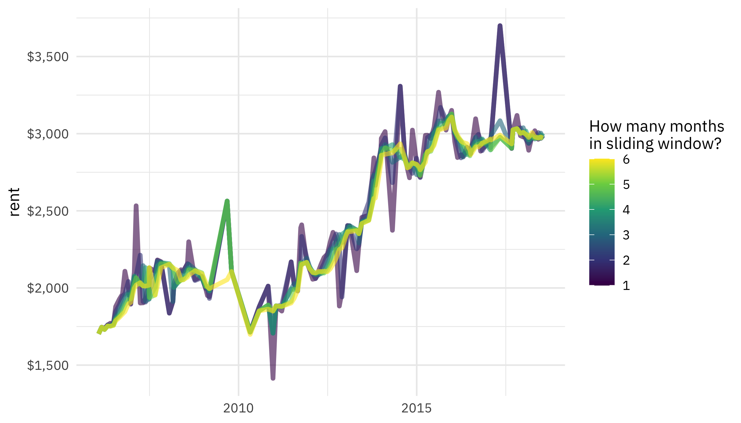
We see smoother change as we aggregate with larger windows, just like we would expect!